Could you be plotting the same phase portrait twice instead, the one for $m=1/4$, instead of plotting two different ones for $m=1/4$ and $m=-1/8$?
I used the following little python script I wrote to help me draw phase portraits of planar vector fields:
import numpy as np
import matplotlib.pyplot as plt
from scipy.integrate import solve_ivp
def solve_IVP(vector_field, x_in, y_in, t_stop, resolution):
    s_0 = 0
    s_1 = t_stop
    y0 = np.array([x_in, y_in])
    t_span = np.linspace(s_0, s_1, num=resolution)
    sol = solve_ivp(vector_field, [s_0, s_1], y0, method='Radau', t_eval=t_span)

    return  sol.t, sol.y
def plot_dynamics_and_multi_traj1(vector_field, IVPs, x_left, x_right, x_res, y_down, y_up, y_res, density, normalized):
    '''
    vector_field = the function defining the vector field V to be integrated:
                   input: x and y (arrays of) coordinates
                   output: a tuple of (arrays of) V_x and V_y calculated coordinates
    IVP = array of arrays, each row contains:
       [x_initial,
        y_initial,
        t_stop = time to stop,
        number of discrete points in the time interval from [0, t_stop] (as float)]
    x_res = number of nodes on the x-axis
    y_res = number of nodes on the y-axis
    density = density of blue background trajectories to be drown
    normalized = set to False, unless you want to integrate the unit-normalized
                 vector field, aligned with the original vector field.

    '''
    if normalized:
      def vf(t, y):
        v = np.array( vector_field(y[0], y[1]) )
        return v / np.sqrt(v.dot(v))
else:
  def vf(t, y):
      return np.array(vector_field(y[0], y[1]))

fig, ax = plt.subplots()
ax.set_aspect('equal')

x_min = x_left
x_max = x_right
y_min = y_down
y_max = y_up

for IVP in IVPs:
   x_in = IVP[0]
   y_in = IVP[1]
   t_stop = IVP[2]
   res_IVP = int(IVP[3])
   sol = solve_IVP(vf, x_in, y_in, t_stop, res_IVP)
   x_min = min(min(sol[1][0,:]), x_min)
   x_max = max(max(sol[1][0,:]), x_max)
   y_min = min(min(sol[1][1,:]), y_min)
   y_max = max(max(sol[1][1,:]), y_max)
   ax.plot(sol[1][0,:], sol[1][1,:], 'r')
   ax.set_aspect('equal')

x, y = np.meshgrid(np.linspace(x_min, x_max, x_res),
                   np.linspace(y_min, y_max, y_res))

Vx, Vy = vector_field(x, y)

if type(Vx) != object:
    Vx = Vx * np.ones(x.shape, dtype=float)
if type(Vy) != object:
    Vy = Vy * np.ones(x.shape, dtype=float)

ax.streamplot(x, y, Vx, Vy, density=density)

plt.grid()
plt.show()

return None
and applied it to your vector field
$$\vec{\text{VF}}(x, y) \, =\, y \, \frac{\partial}{\partial x} \, +\,\big( -x^3- y + m\, y \, \big)\frac{\partial}{\partial y}$$
# equations defining the vector field:
def VF(x, y):
  return (y,  -x**3 - y - m*x)
I set up a list of starting points selected horizontally over and under the x-horizontal axis (initial value parameters IVPs):
# bifurcation parameter
m = 1/2
how many equally spaced nodes to select along the x-axis
x_res = 100
how many equally spaced nodes to select along the y-axis
y_res = x_res
the right endpoint of the plot on the x-axis
x_size=0.5
the top endpoint of the plot on the y-axis
y_size=0.3
for how much time to integrate the trajectories
stop_time = 12
number of points along each trajectory to be used for integrating the equations
sample_points_on_trajectory = 500
setting up the initial values:
choose an array of initial points for a finite number of solution trajectories:
set up the x-coordinates of the initial points:
IVPs =np.arange(-x_size, x_size, 2*x_size/10)
IVPs = np.concatenate((IVPs, - IVPs), axis=0)
set up the initial value parameters:
row1 = x-coordinates of initial points
row2 = y-coordinates of initial points (left empty for now)
row3 =
IVPs = np.array([IVPs,
                 np.empty(len(IVPs), dtype=float),
                 stop_time * np.ones(len(IVPs), dtype=float),
                 sample_points_on_trajectory * np.ones(len(IVPs), dtype=float)])
initializing row2 = y-coordinates of initial points:
below the x-axis
IVPs[1 , 0:int(IVPs.shape[1]/2)] = - y_size
above the x-axis
IVPs[1, int(IVPs.shape[1]/2): IVPs.shape[1]] = y_size
transpose the initial value parameters:
IVPs = IVPs.T
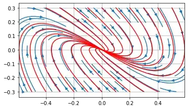
and plotted the following two phase portraits:
$$m = \frac{1}{4}$$
# bifurcation parameter
m = 1/4
plot the phase portrait:
plot_dynamics_and_multi_traj1(VF, IVPs,-x_size, x_size, x_res,
                                       -y_size, y_size, y_res,
                                        density=0.7, normalized=False)
and $$m = -\,\frac{1}{8}$$
# bifurcation parameter
m=-1/8.
plot the phase portrait:
plot_dynamics_and_multi_traj1(VF, IVPs,-x_size, x_size, x_res,
                                       -y_size, y_size, y_res,
                                        density=0.5, normalized=False)
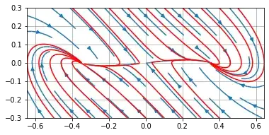
As you can see, when the bifurcation parameter $m$ goes from positive to negative values, the stable equilibrium point changes from being asymptotically stable focus to three equilibria, one saddle point in the middle and two symmetric stable nodes.


