This answer will rely on the same method as the two answers of users curious and Emilio Pisanty, possibly dotting a few i's along the way. In particular, we will pay attention to signs, which play an important role (e.g. Should the swimmer swim upsteam$^1$ or downstream?).
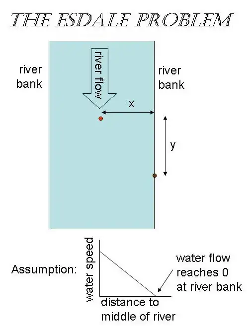
I) In this answer we consider the time-reversed (but equivalent) problem of minimizing the total time $T$ it takes to go from the river shore $(x_i,y_i)=(0,0)$ to a fixed position $(x_f,y_f)=(L,y_f)$ in the middle of the river (in a coordinate system that is stationary wrt. the shore). In other words, we use Eulerian (as opposed to Lagrangian) coordinates. Let the velocity profile of the river be linear
$$v(x)~:=~ \frac{x}{L}V.\tag{1}$$
The velocity of the swimmer is
$$\begin{align}\dot{x}~=~&v_0 \cos\theta > 0,\cr \dot{y}~=~& v_0 \sin\theta + v(x),\end{align}\tag{2}$$
where the angle $\theta\in ]-\frac{\pi}{2},\frac{\pi}{2}[$ is a control parameter. (We assume that bang-bang solutions $|\theta|=\frac{\pi}{2}$ are not relevant.)
II) Let us for convenience go to dimensionless primed coordinates
$$\begin{align} x ~=~& L x^{\prime}, \cr
y ~=~& L y^{\prime},\cr
t ~=~& \frac{L}{v_0} t^{\prime},\cr
V ~=~& v_0 V^{\prime}.\end{align}\tag{3}$$
We will not write the primes explicitly from now on. This has the effect of scaling the parameters
$$ L~=~1~=~v_0.\tag{4}$$
(The dimensionful parameters $L$ and $v_0$ can easily be recovered in the end by dimensional analysis.)
III) Noticing the positive $x$-velocity (2), we next reparametrize the problem in terms of $x$ rather than $t$, i.e. $x$ will play the role of a 'clock' for the swimmer. This has the added benefit that the final 'time' $x_f=L=1$ is fixed (as opposed to free), which makes the optimal control problem simpler. We also pick a new control parameter
$$ s(x)~:=~\sin\theta(x)~ \in~ ]-1,1[.\tag{5}$$
IV) The total time becomes
$$\begin{align} T~=~&\int_0^T \!dt\cr
~=~& \int_0^1 \! \frac{dx}{\dot{x}} \cr
~=~& \int_0^1 \! \frac{dx}{\sqrt{1-s^2}}.\end{align} \tag{6}$$
The $y$-coordinate is (with the slight abuse of notation where the upper integration limit $x$ and integration variable $x$ are given the same name)
$$\begin{align} y(x)~=~&\int_0^{y(x)} \!dy\cr
~=~& \int_0^x \!dx \frac{dy}{dx} \cr
~=~& \int_0^x \!dx \frac{\dot{y}}{\dot{x}} \cr
~=~& \int_0^x \!dx \frac{s+v}{\sqrt{1-s^2}}. \end{align}\tag{7}$$
The final $y$-coordinate is similarly
$$ y_f~=~\int_0^1 \! dx\frac{s+v}{\sqrt{1-s^2}}. \tag{8}$$
V) The task is to minimize (6) keeping in mind the constraint (8). The 'action' becomes
$$ \begin{align}S ~=~& T +\lambda\left(y_f-y(x\!=\!L)\right) \cr
~=~&\int_0^1 \!dx~ L,\end{align}\tag{9} $$
with Lagrangian
$$\begin{align} L
~=~&\frac{1}{\sqrt{1-s^2}} + \lambda \left[\frac{s+v}{\sqrt{1-s^2}} -y_f\right]\cr
~=~& \frac{1+\lambda(s+v)}{\sqrt{1-s^2}}-\lambda y_f. \end{align}\tag{10}$$
Here $\lambda$ is an $x$-independent Lagrange multiplier. The Euler-Lagrange equation reads
$$ \begin{align} 0 ~\approx~&\frac{\partial L}{\partial s}
~=~ \frac{s(1+\lambda v)+\lambda}{(1-s^2)^{\frac{3}{2}}}
\cr \Updownarrow & \cr
s~\approx~& -1/w,\end{align}\tag{11}$$
where we have defined
$$\begin{align} w(x)~:=~&v(x)+\mu, \cr
\mu~:=~&\frac{1}{\lambda}.\end{align}\tag{12} $$
The $\approx$ symbol in eq. (11) means equality modulo equation of motion.
VI) We see from the eom (11), that the optimal strategy for the cosecant $\csc\theta(x)\approx-w(x)$ is an affine (and therefore monotonic) function of $x$. E.g. it is not optimal to first swim upstream and later downstream. Moreover, swimming straight into the river $s=0$ will never be an optimal strategy (apart from the trivial case $V=0=y_f$). Let us therefore exclude $s=0$ in what follows. Hence the control double inequality (5) is divided into swimming downstream or swimming upstream$^1$,
$$ 0~<~s~<~1 \quad \vee \quad -1~<~s~<~0, \tag{13}$$
or equivalently,
$$ w ~< ~ -1 \quad \vee \quad w~>~1,\tag{14} $$
or equivalently,
$$ \mu ~<~ -(V+1) \quad \vee \quad \mu ~>~1, \tag{15} $$
or equivalently,
$$ -\frac{1}{V+1} ~<~ \lambda~<~0\quad \vee \quad 0~<~\lambda ~<~1,\tag{16}$$
respectively. In particular, we conclude that the control parameter $s$ and the Lagrange multiplier $\lambda$ have opposite signs,
$$ -{\rm sgn}(s)~=~{\rm sgn}(w)~=~{\rm sgn}(\mu)~=~{\rm sgn}(\lambda).\tag{17}$$
VII) The minimal total time becomes
$$\begin{align} T ~\stackrel{(6)+(11)}{\approx}&
\int_{x=0}^{x=1} \!\frac{dw}{V} \frac{|w|}{\sqrt{w^2-1}}\cr
~=~& \frac{1}{V} \left[{\rm sgn}(w) \sqrt{w^2-1}\right]_{x=0}^{x=1}\cr
~=~& \frac{{\rm sgn}(\mu)}{V} \left(\sqrt{(V+\mu)^2-1}-\sqrt{\mu^2-1}\right) \end{align}\tag{18}. $$
The optimal $y$-coordinate is
$$\begin{align} y(x)~\stackrel{(8)+(11)}{\approx}&
\int_{x=0}^{x=x} \! \frac{dw}{V}\frac{v|w|-{\rm sgn}(w)}{\sqrt{w^2-1}} \cr
~=~& \int_{x=0}^{x=x} \! \frac{dw}{V}{\rm sgn}(w)\frac{(w-\mu)w-1}{\sqrt{w^2-1}} \cr
~=~& \int_{x=0}^{x=x} \! \frac{dw}{V}{\rm sgn}(w) \sqrt{w^2-1}
- \mu T \cr
~=~& \frac{1}{2V} \left[|w| \sqrt{w^2-1}
-{\rm sgn}(w) {\rm arcosh}(w)\right]_{x=0}^{x=x}
- \mu T \cr
~=~& \frac{1}{2V} \left[{\rm sgn}(w)\left( (w-2\mu) \sqrt{w^2-1}- {\rm arcosh}(w)\right)\right]_{x=0}^{x=x} \cr
~=~&\frac{{\rm sgn}(\mu)}{2V} [ (v(x)-\mu) \sqrt{(v(x)+\mu)^2-1}+\mu\sqrt{\mu^2-1} \cr
& -{\rm arcosh}(v(x)+\mu)+{\rm arcosh}(\mu)]. \end{align}\tag{19}$$
The optimal final $y$-coordinate is similarly
$$\begin{align} y_f ~=~&\frac{{\rm sgn}(\mu)}{2V} [ (V-\mu) \sqrt{(V+\mu)^2-1}+\mu\sqrt{\mu^2-1} \cr
& -{\rm arcosh}(V+\mu)+{\rm arcosh}(\mu)]. \end{align}\tag{20}$$
Eq. (20) is an equation for the (reciprocal) Lagrange multiplier $\mu$ in terms of $y_f$ and $V$. The solution for $\mu$ should then be inserted in the formula (18) for $T$ to get the sought-for final result. However in general there is no hope to solve the transcendental eq. (20) in closed form. But one may find explicit solutions in certain limits. For instance in the weak current limit $V\ll 1$.
VIII) Let us finally study the weak current limit $V\ll 1$. In that limit the minimal total time is
$$\begin{align}0~<~T~\simeq~& {\rm sgn}(\mu)\left[
\frac{\mu}{\sqrt{\mu^2-1}}
-\frac{1}{2(\mu^2-1)^{\frac{3}{2}}}V
+\frac{\mu}{2(\mu^2-1)^{\frac{5}{2}}}V^2
+{\cal O}(V^3)\right]\cr
~\stackrel{(23)}{\simeq}~& -\mu z +\frac{z^3}{2}V+{\cal O}(V^2) ,\end{align}\tag{21}$$
and the optimal final $y$-coordinate is
$$\begin{align} y_f~\simeq~& {\rm sgn}(\mu)\left[
-\frac{1}{\sqrt{\mu^2-1}}
+\frac{\mu^3}{2(\mu^2-1)^{\frac{3}{2}}}V
+\frac{1-4\mu^2}{6(\mu^2-1)^{\frac{5}{2}}}V^2
+{\cal O}(V^3) \right] \cr
~\stackrel{(23)}{\simeq}~& z +\frac{(-\mu z)^3}{2}V+{\cal O}(V^2)\cr
~\stackrel{(21)}{\simeq}~& z +\frac{T^3}{2}V+{\cal O}(V^2) .\end{align}\tag{22}$$
Here we have introduced a convenient expansion parameter
$$\begin{align} z~:=~ -\frac{{\rm sgn}(\mu)}{\sqrt{\mu^2-1}}, \qquad
{\rm sgn}(z)~=~-{\rm sgn}(\mu). \tag{23}
\end{align} $$
Eq. (22) may be inverted
$$ z ~\simeq~y_f-\frac{T^3}{2}V+{\cal O}(V^2) , \tag{24}$$
$$ |\mu|~\simeq~ \sqrt{1+y_f^{-2}} -{\rm sgn}(\mu) \frac{1+y_f^{-2}}{2}V +{\cal O}(V^2) . \tag{25}$$
Thus we arrive at a weak limit formula for the minimal time
$$ T~\simeq~ \sqrt{y_f^2+1} - {\rm sgn}(\mu)\frac{|y_f|^3}{2}V+{\cal O}(V^2). \tag{26} $$
The sign ${\rm sgn}(\mu)=-{\rm sgn}(z)$ should be determined from eq. (24).
As a quick check we see that eq. (26) reproduces Pythagoras' formula $(v_0T)^2\simeq y_f^2+L^2$ when there is no current $V=0$ at all.
From eqs. (22) or (24) we deduce that $z< y_f$. On one hand, if $y_f<0$ is upstream, then $z>0$ and $\mu<0$, meaning that the swimmer should not surprisingly swim upstream. On the other hand, if $y_f>0$ is downstream, for the swimmer to determine whether he should swim up- or downstream$^1$, he must first determine the sign of $z$ from eq. (24).
--
$^1$ Here we mean swimming upstream in the steering sense. The resulting motion may be downstream due to the river flow.