Fourier integral provides only a particular solution of the inhomogeneous equation, whereas the full solution consists of a particular solution of the inhomogeneous equation plus the general solution of the homogeneous equation (since the latter can always be added to the inhomogeneous solution.) Retarded Green's function is obtained as a solution with specific boundary/initial conditions:
$$
G(t,t')=0\text{ for } t<t'.
$$
In fact, when solving a problem with initial conditions, it is more appropriate to use Laplace rather than Fourier transform, which explicitly incorporates the initial conditions.
Retarded Green's function from Fourier integral
My question is: why doesn't this Fourier integral naturally yield 0 for t<0?
The Green's functions (retarded, advanced, etc.) of a harmonic oscillator satisfy equation
$$
\partial_t^2G(t,t')+2\gamma\partial_t G(t,t')+\omega_0^2G(t,t')=\delta(t-t').$$
Due to time-translational invariance $G(t,t')=G(t-t')$, so we can solve without loss of generality
$$
\ddot{G}(t)+2\gamma\dot{G}(t)+\omega_0^2G(t)=\delta(t).$$
Fourier representations for the Green's function and delta function are
$$
G(t)=\int\frac{d\omega}{2\pi}e^{i\omega t}\tilde{G}(\omega),
\delta(t)=\int\frac{d\omega}{2\pi}e^{i\omega t}
$$
Substituting these to the equation results in
$$
\int\frac{d\omega}{2\pi}e^{i\omega t}\left[(i\omega)^2+2\gamma i\omega +\omega_0^2\right]\tilde{G}(\omega)=
\int\frac{d\omega}{2\pi}e^{i\omega t}\\
\Rightarrow \left[-\omega^2+2i\gamma \omega +\omega_0^2\right]\tilde{G}(\omega)=1.
$$
Thus, we have
$$
\tilde{G}(\omega)=\frac{1}{-\omega^2+2i\gamma \omega +\omega_0^2}=
\frac{-1}{(\omega -i\gamma)^2-\omega_0^2+\gamma^2}=
\frac{-1}{(\omega -i\gamma+\sqrt{\omega_0^2-\gamma^2})(\omega -i\gamma-\sqrt{\omega_0^2-\gamma^2})}
$$
This is the expression for the Green's function provided in the Q. I spelled exactly several trivial steps to assure that the Q. did not result from a mistake in these derivations, as the choice of the sign in the complex exponent that leads to this expression seems to me somewhat unusual (speaking from a quantum background.)
We now can evaluate the inverse Fourier transform:
$$
G(t)=-\int_{-\infty}^{+\infty}\frac{d\omega}{2\pi}
\frac{e^{i\omega t}}{(\omega -i\gamma+\sqrt{\omega_0^2-\gamma^2})(\omega -i\gamma-\sqrt{\omega_0^2-\gamma^2})}
$$
The integrand has two poles in the upper complex half-plane:
$$
\omega_{1,2}=\pm \sqrt{\omega_0^2-\gamma^2} + i\gamma,
$$
whereas the integration runs along the real axis. We could try to close the contour by an arc in one of the half-planes and use the residue theorem (image source):
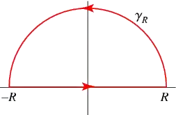
On the arc frequency has real and complex parts: $\omega=\omega'+i\omega''$, so that the complex exponent becomes
$$
e^{i\omega t}=e^{i\omega' t-\omega'' t}.
$$
Thus, if $t>0$ and we close the contour in the upper half plane ($\omega''>0$), the contribution from the arc will vanish, and the residue theorem gives the value of the integral over the real axis. On the other hand, closing the contour in the low half-plane would produce a divergent contribution, and hence is a no-go.
The situation is the opposite for $t<0$ - we must close the contour in the lower half plane.
Now, since the integrand has no poles in the lower half-plane, the residue theorem for $t<0$ gives zero result:
$$
G(t)=0,\text{ if } t<0.
$$
For $t>0$ we have to calculate the residues from the two poles, obtaining
$$
G(t)=\frac{-1}{2\pi}2\pi i \left[\frac{e^{i(i\gamma+\sqrt{\omega_0^2-\gamma^2})t}}{2\sqrt{\omega_0^2-\gamma^2}}+
\frac{e^{i(i\gamma-\sqrt{\omega_0^2-\gamma^2})t}}{-2\sqrt{\omega_0^2-\gamma^2}}
\right]=\\
\frac{-i}{2\sqrt{\omega_0^2-\gamma^2}}
\left[e^{-\gamma t+i\sqrt{\omega_0^2-\gamma^2}t} -
e^{-\gamma t-i\sqrt{\omega_0^2-\gamma^2}t}\right]=\\
\frac{e^{-\gamma t}\sin\left(\sqrt{\omega_0^2-\gamma^2}t\right)}{\sqrt{\omega_0^2-\gamma^2}}
$$
That is
$$
G(t)=\begin{cases}
\frac{e^{-\gamma t}\sin\left(\sqrt{\omega_0^2-\gamma^2}t\right)}{\sqrt{\omega_0^2-\gamma^2}},
\text{ if } t>0,\\
0,\text{ if } t<0
\end{cases}
=
\Theta(t)\frac{e^{-\gamma t}\sin\left(\sqrt{\omega_0^2-\gamma^2}t\right)}{\sqrt{\omega_0^2-\gamma^2}},
$$
which is the retarded Green's function in the Q.
For instance, with $F(t)=\cos\omega t$, integrating directly over the $\delta$ functions in $\tilde{F}$ (rather than by contour integration) gives the steady state solution, valid for all $t$ positive and negative.
(emphasis mine)
The reason for that is that in case of $F(t)=\cos\omega t$ we have $t'\rightarrow -\infty$, so all the times $t$ are positive. It would be different, if the perturbation is turned on at a specified instant, e.g.,
$$
F(t)=\Theta(t-t')\cos\omega t
$$
(but of course the Fourier integral in this case is less trivial to calculate.)
