QFT is difficult, unfortunately. Usually in a 1st pass in QFT, one is interested in computing different cross sections $d\sigma$. These differential cross sections can be related to the square of the scattering amplitude $\mathcal M$. For a scattering event of $A+B\rightarrow 1\ldots m$ distinguishable particles in $n$ spatial dimensions one has $$d\sigma=\frac{1}{2E_AE_B|v_A-v_B|}\prod_{f=1}^m\frac{d^np_f}{(2\pi)^n2E_f}|\mathcal M(A+B\rightarrow\sum_i p_i)|^2(2\pi)^{n+1}\delta^{(n+1)}(p_A+p_B-\sum_i p_i);$$ see, e.g., Ch. 4 of Peskin and Schroeder.
The scattering amplitude $\mathcal M$ is in turn related to the overlap of the asymptotic $in$ state $|p_Ap_B;in\rangle$ and the asymptotic $out$ state $|p_1\ldots p_m;out\rangle$, $$i\mathcal M(p_1\ldots p_m; p_Ap_B)(2\pi)^{n+1}\delta^{(n+1)}(p_A+p_B-\sum_ip_i)\equiv\langle p_1\ldots p_m;out|p_Ap_B;in\rangle.$$
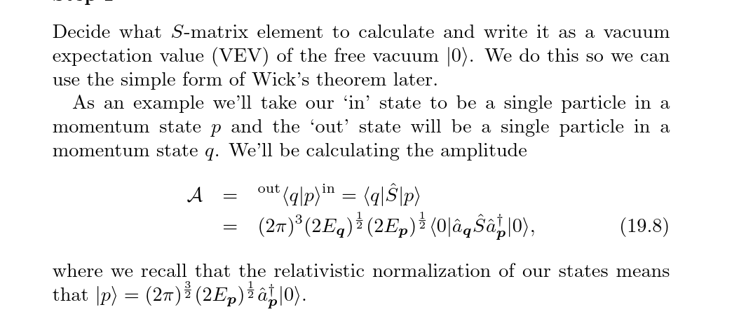
One may then compute these asymptotic $in$ and $out$ states using LSZ reduction. For a theory of scalar fields, one has $$\langle \rho_1\ldots \rho_m;out|\kappa_1\ldots\kappa_\ell;in\rangle = \int d^{n+1} x_1\cdots d^{n+1}x_md^{n+1}y_1\cdots d^{n+1}y_\ell e^{i\sum_i^m\rho_i\cdot x_i}e^{-i\sum_j^\ell \kappa_j\cdot y_j}(i)^{m+\ell}\prod_{i=1}^m(\Box_{x_i}+m_{phys}^2)\prod_{j=1}^\ell(\Box_{y_j}+m_{phys}^2)\langle\Omega|T\{\phi'(x_1)\cdots\phi'(x_m)\phi'(y_1)\cdots\phi'(y_\ell)\}|\Omega\rangle \\ = \prod_{i=1}^m \frac{\rho_i^2-m_{phys}^2}{i}\prod_{j=1}^\ell\frac{\kappa_j^2-m_{phys}^2}{i}\tilde G'(\rho_1\ldots\rho_m;-\kappa_1\ldots -\kappa_\ell),$$ where $$\tilde G'(\rho_1\ldots\rho_m;-\kappa_1\ldots -\kappa_\ell)\equiv\int d^{n+1} x_1\cdots d^{n+1}x_md^{n+1}y_1\cdots d^{n+1}y_\ell e^{i\sum_i^m\rho_i\cdot x_i}e^{-i\sum_j^\ell \kappa_j\cdot y_j}G'(x_1\ldots x_m,y_1\ldots y_\ell)$$ is the Fourer transform of the $n+m$-point "renormalized" Green function $$G'(x_1\ldots x_m,y_1\ldots y_\ell)\equiv\langle\Omega|T\{\phi'(x_1)\cdots\phi'(x_m)\phi'(y_1)\cdots\phi'(y_\ell)\}|\Omega\rangle.$$ I've put renormalized in quotes because the field $\phi'$ is renormalized, but may not necessarily coincide with the renormalization choice taken. In particular, $\phi'$ must satisfy 1) $\langle\Omega|\phi'(x)|\Omega\rangle=0$; i.e. there's no vacuum expectation value (VEV) for $\phi'$ (no tadpole diagrams) and 2) $\langle\kappa|\phi'(x)|\Omega\rangle = e^{i\kappa\cdot x}$; i.e. $\kappa$ corresponds to our usual notion of a normalized plane wave. See, e.g., Coleman's Harvard Lecture Notes (free on the arXiv!) or Itzykson and Zuber.
One of the major points of LSZ above is that interacting fields are very complicated; even the interacting vacuum, $|\Omega\rangle$, is very complicated and should be distinguished form the free field vacuum $|0\rangle$. The free field vacuum is empty, but the interacting vacuum has particle--anti-particle pairs popping in and out of existence all the time. For tree level processes, which you're probably interested in at this point, things simplify considerably because one doesn't need to worry about renormalization, which only kicks in once there are loops.
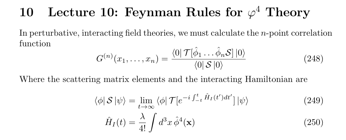
Now one needs to compute the nasty $n+m$-point GF that's made up of horrific fully interacting fields in the Heisenberg Picture. The next and final trick is to use the Gell-Mann--Low theorem (see again Ch. 4 of Peskin). The GM-L theorem allows one to see that a Heisenberg Picture operator matrix element may be expressed in terms of Interaction Picture operator matrix elements via $$\langle\Omega|\phi_H(x)|\Omega\rangle = \lim_{T\rightarrow\infty(1-i\epsilon)}\frac{\langle0|T\{\phi_I(x)e^{-i\int_{-T}^Tdt'H_I(t')}\}|0\rangle}{\langle0|T\{e^{-i\int_{-T}^Tdt'H_I(t')}\}|0\rangle}.$$ Mercifully we can evaluate the expression on the RHS since all the fields are in the Interaction Picture and we may expand the time ordered exponential into a Dyson Series. This last expression is what I believe you're seeing in the lecture notes.