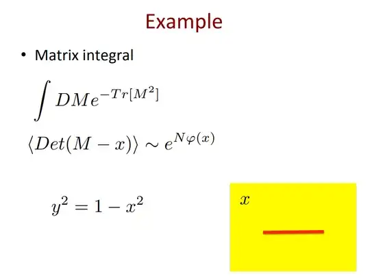
The standard definition of the integral, for $N \times N$ Hermitian matrices, is:
$$
Z = \frac{1}{\textrm{vol}(U(N))}\int DM e^{- \textrm{Tr} M^2}
$$
The normalization factor accounts for the $U(N)$ internal symmetry of the action. This can be interpreted in two ways: we can regard it as the path integral for a 0+0 dimensional QFT of matrices, or we can think of this as describing sort of Gaussian distribution over the space of Hermitian matrices. The measure (a sort of Haar measure) is defined as:
$$
DM = \prod_i^N dM_{ii} \prod_{i<j}^N d(\textrm{Re} M_{ij})d(\textrm{Im} M_{ij})
$$
Taking the first viewpoint, we can fix the gauge to "diagonal" gauge by a unitary transformation. Then the trace becomes a sum over eigenvalues, but the measure has a non-trivial Jacobian:
$$
\textrm{Tr} M^2 = \sum_{i = 1}^N \lambda_i^2;\quad DM = DU\prod_i^N d\lambda_i \prod_{i<j}^N (\lambda_i - \lambda_j)^2
$$
$DU$ integrates to cancel the normalization.
2)
The new quantity in the measure $\prod (\lambda_i - \lambda_j)^2$ is called the Vandermonde determinant (or rather, its square). It implies that in the space of matrix-valued field configurations, if two eigenvalues coincide the path integral measure has no support there. So eigenvalues tend to repel each other from sharing the same value (in other words, there is a larger amplitude for separated eigenvalues).
In fact, one can show that the eigenvalues behave exactly like a gas of non-interacting fermions, and many aspects of the theory can then be solved exactly. Just as in statistical mechanics, we need to take the large $N \to \infty$ limit for this to be tractable with methods of thermodynamics. You can read more about this in any review on matrix models, this one by Mariño includes details on non-perturbative effects in these theories: https://arxiv.org/abs/1206.6272.
3)
There are two relations you could be referring to: the correspondence of matrix integrals and 2d gravity, or the analytic structure of matrix models. If it is the first, I direct you to https://arxiv.org/abs/1903.11115 and references therein. The latter (and the one which Maldacena is talking about) is quickly summarized by the following.
To sketch the relation, consider the problem introduced above as $N \to \infty$. This is the planar limit (up to what you also have to do to the coupling). Then I can make sense of an eigenvalue distribution $\lambda(x)$ and define a function $y(\lambda)$ by $\partial x/\partial\lambda = y(\lambda)$. This function is the so-called "spectral curve". Through this one can define an analytic function
$$
F(z) = \int_C dx \frac{y(x)}{z-x}
$$
where $C$ is some (possibly disconnected) contour on which the spectral curve is supported. This function $F(z)$ will be analytic away from branch cuts where $z \in C$. For a potential with $k$ critical points, the function $F(z)$ has a domain of analyticity away from $k$ branch cuts in the complex plane. This domain can be considered a multi-sheeted Riemann surface, where $F(z)$ is well-defined. Then techniques from the theory of Riemann surfaces allow us to determine $F(z)$ (it is more or less a Riemann-Hilbert problem) and hence the distribution of eigenvalues, from which we can reconstruct some of the dynamics and combinatorics.
4)
This part is not as clear to me, but I can offer the explanation that I have heard. The idea is that black holes are very complicated, chaotic quantum systems with many degrees of freedom. This makes sense: a solar mass black hole has entropy $S \sim 10^{77}$. The number of degrees of freedom goes like $N \approx e^S$, which is astronomically large. Many-component quantum systems are often described by density matrices:
$$\rho = \sum_{x \in \mathcal{H}} |x\rangle \langle x|$$
over all states $x$. Density matrices are Hermitian operators. If each degree of freedom is one quantum bit, the matrix elements describe an $N \times N$ Hermitian matrix with $N >> 1$. If the dynamics are chaotic, one can compute aspects of the dynamics by considering this situation to be a large $N$ random matrix model. This and more is outlined in https://arxiv.org/abs/1611.04650, and is the subject of much recent work.
