1

I am trying to understand renormalization in Wilson approach.

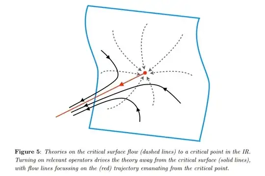
There's cool picture, which demonstrates flow of theories in IR:

So, if one interested in UV limit, one need reverse flow and flow in this reverse direction.

As it clear from picture, this procedure can be done only for red line. Dashed or solid line will lead us in UV to infinite values of couplings.

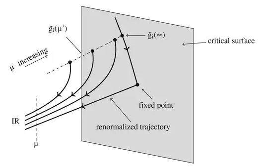
But in 6 Lectures on QFT, RG and SUSY there's the picture, which illustrate continuous limit:

As I understand, the idea is in construction on some lines of theories, that will lead to finite couplings values on infinite energy scale.

But this looks incorrect, because in finite scale $\mu$ these theories have different IR limits.

So, I don't understand, how to take continuous limit, if effective theory doesn't lie on renormalized trajectory?
Nikita
  • 5,757
  • 3
  • 18
  • 51

1 Answers1

4

I explained all this in I hope sufficient detail at

What is the Wilsonian definition of renormalizability?

and I urge the OP to read it. However, let me give some quick remarks here.

There is not much to say about the first picture which just shows how the RG flow looks like near the UV fixed point that one is trying to perturb in order to construct a new family of QFTs in the continuum. Except one could say that in order to properly interpret the picture, one has to keep in mind that the coordinates in the picture are dimensionless couplings and not dimensionful ones typically used in HEP. The second picture deserves more comments as it provides a pedagogical cartoon for how to take a continuum limit. In "continuum limit" the important word here is "limit". When the dust settles, one has removed the cutoff etc., the final product or continuum QFT is the curve labelled "renormalized trajectory". It is obtained as a limit of other curves. For each $\mu'$, you pick a starting point $\tilde{g}_i(\mu')$ and you run the RG from there. That gives you a curve. If the starting points are well chosen, these curves will converge to the limiting curve "renormalized trajectory".

Note that the picture illustrates a very general approach (standard plus more exotic constructions). The simplest and most common way (standard construction) to pick the starting points is as points on the tangent at the fixed point to the "renormalized trajectory". Namely, as $\mu'\rightarrow \infty$, the initial values $\tilde{g}_i(\mu')$ will converge to the fixed point itself. Think, for example, of a Gaussian fixed point, and the $\tilde{g}_i(\mu')$ only containing relevant terms (in fact only one if the 1st picture is to be trusted as saying there is only one relevant direction). The more exotic construction suggested by the 2nd picture is when the $\tilde{g}_i(\mu')$ converge not to the fixed point but to a point on the stable manifold of that fixed point. If you want an example where this "exotic" construction done in a mathematically rigorous and nonperturbative way, see Theorems 5 and 6 in Section 9 of the article

https://arxiv.org/abs/1302.5971