Can the Euler-Lagrange equations be derived from an infinitesimal Principle of Least Action?

Question

The Euler-Lagrange equations can be derived from the Principle of Least Action using integration by parts and the fact that the variation is zero at the end points.

This has a mystical air about it, with the system somehow "sniffing" out all possible paths in the distant future and choosing the one that minimizes the action. An infinitesimal version would make the method less mystical in this sense, and so I would like to ask:

Can the Euler-Lagrange equations be derived from an infinitesimal principle of least action?

Answer 1

The differential equations do the same thing: after integration you obtain a solution with "two" arbitrary constants. It means you obtain a whole two-parametric family of possible solutions (curves). Fixing endpoints reduces the solution to one unique curve. It has the property to obey the differential equations (=> minimises the action) and to pass through the given endpoints.

Answer 2

Let us just consider point mechanics$^1$

$$ S[q]~:=~\int_{t_i}^{t_f}\!dt~ L, \qquad L~=~L(q,\dot{q},t)$$

to be concrete, where $t_i$ and $t_f$ denote initial and final time, respectively; and we have imposed some appropriate boundary conditions.

I guess OP is asking his question(v1) because of the apparent teleology of the stationary action principle, as also discussed in this Phys.SE answer.

One can get a local stationary action principle as follows: If one assumes that there exists a possibly very small (but finite) constant $\epsilon>0$ (of dimension time), such the stationary action principle holds for all $t_i$ and $t_f$ with $|t_f-t_i|<\epsilon$, then one would still be able to derive the Euler-Lagrange equations (via the standard derivation).

By choosing $\epsilon$ much smaller than all the characteristic time scales of the physical problem, this would for all practical purposes be "an infinitesimal stationary action principle".

But at the philosophical level, if OP felt uneasy about the apparent teleology before, he would probably still feel uneasy about the above $\epsilon$-local stationary action principle, no matter how small $\epsilon$ is chosen.

I agree with Nick Kidman's comment above, that "an infinitesimal stationary action principle", in its manifestly infinitesimal form, would just constitute the Euler-Lagrange equations themselves.

--

$^1$The field-theoretic generalization is straightforward.

Answer 3

The infinitesimal case eliminates the apparent tetology because we can predict where the system will be at time $dt$ in the future from $dq = \dot q dt$.

Let's start with the one dimensional case. To vary the path over an infinitesimal time, we need at least two infinitesimal time intervals where $\dot x$ is varied by $\delta\dot x_1$ over $dt_1$, and then in the opposite sense $\delta\dot x_2$ over $dt_2$. Thus it ends up at the predicted fixed position $\dot x(dt_1+dt_2)$

The infinitesimal action is then simply the Riemann sum over $dt_1$ and $dt_2$ $$L_t = L(x,\dot x ,t),\,L_{dt1} = L(x+\dot xdt_1,\dot x,t+dt_1),\, L_{\delta \dot x dt1} = L(x+(\dot x+ \delta \dot x_1)dt_1,\dot x,t+dt_1)$$

$$ ds = L_tdt_1 + (L_t + \frac {\partial L_{dt1}}{\partial x}\dot xdt_1)dt_2$$

$$ ds+ \delta ds = (L_t + \frac {\partial L_t} {\partial \dot x}\delta \dot x_1)dt_1 + (L_{\delta\dot x dt1} + \frac {\partial L_{\delta \dot x dt1}} {\partial \dot x}\delta \dot x_2 + \frac {\partial L_{\delta \dot x dt1}} {\partial x}(\dot x+\delta\dot x_1)dt_1)dt_2$$

Since the variation in position over $dt_1$ must be compensated by that over $dt_2$, then $\delta \dot x_1dt_1 = - \delta \dot x_2dt_2$, so that

$$ \begin{align*}\delta ds &= (\frac {\partial L_t} {\partial \dot x}\delta \dot x_1- \frac {\partial L_{\delta\dot x dt1}} {\partial \dot x}\delta \dot x_1 )dt_1 + \frac {\partial L_{\delta \dot x dt1}} {\partial x}\delta\dot x_1dt_1dt_2\\ &=0\\ &= -\frac{\frac {\partial L_{\delta\dot x}} {\partial \dot x}-\frac {\partial L_t} {\partial \dot x}}{dt_2} +\frac {\partial L_{\delta \dot x dt1}} {\partial x}\\ &= -\frac {d}{dt}\frac {\partial L}{\partial \dot x} + \frac{\partial L}{\partial x}\end{align*}$$

Obviously this generalises to any number of coordinates since the infinitesimal action can be varied independently for each $q_i$.

Answer 4

I know this question was posted 10 years ago. I checked your user profile, and by the looks of it you are still visiting physics.stackexchange, so I decided to go ahead and post this answer.

Indeed it is possible to derive the Euler-Lagrange equation using differential operations only.

In Oktober 2021 I posted an answer with a discussion of Hamilton's stationary action, with among other things a derivation of the Euler-Lagrange equation using differential operations only.

The reason why that is possible was actually recognized long before Calculus of Variations was developed.

As we know, Johann Bernoulli issued the Brachistochrone challenge in the 1690's. (In retrospect it is recognized that the Brachistochrone problem is the type of problem that calculus of variation is suited to. Actual development of calculus of variations occurred in the 1780's)

Among the few mathematicians of the time that were able to solve the Brachistochrone problem was Jacob Bernoulli, Johann's older brother.

Jacob Bernoulli recognized a crucial feature of the brachistochrone problem, and he presented that feature in the form of a lemma:

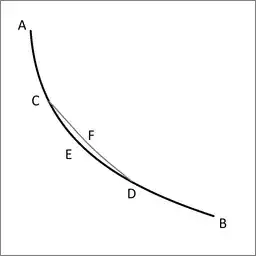
Let ACEDB be the desired curve along which a heavy point falls from A to B in the shortest time, and let C and D be two points on it as close together as we like. Then the segment of arc CED is among all segments of arc with C and D as end points the segment that a heavy point falling from A traverses in the shortest time. Indeed, if another segment of arc CFD were traversed in a shorter time, then the point would move along AGFDB in a shorter time than along ACEDB, which is contrary to our supposition.

(Acta Eruditorum, May 1697, pp. 211-217)

Rephrasing:
Take the solution to the Brachistochrone problem, and take an arbitrary subsection of that curve. That subsection is also an instance of solving the brachistochrone problem. This is valid at any scale; down to arbitrarily small scale.

Therefore the following strategy will work:
Divide the curve in concatenated subsections, and formulate an equation that is valid for all the subsections concurrently.

Generalizing: In order for the derivative of $\int_{x_2}^{x_1}$ to be zero: divide the domain in concatenated subsections, and set the condition: for every subsection between $x_1$ and $x_2$ the derivative of the corresponding integral must be zero concurrently. Take the limit of infinitisimally short subsections.

When you see the Euler-Lagrange equation being derived using integration by parts your first reaction is: "Hang on, this derivation results in a differential equation, what happened to the integration?"

The reason the integration operation can be eliminated: calculus of variations is about infinitisimals to begin with.

The condition that the derivative must be zero applies for sections down to infinitisimally small length, and from there it applies for concatenated subsections concurrently.

Concatenable

Jacob's lemma, and the generalized form of it, are applicable when the problem is such that it can be subdivided in concatenable subsections.

In mathematics there are also classes of problems such that subdivision in concatenable subsections is not available. An example of that is the traveling salesman problem.