Following J.R.Taylor's Classical Mechanics
Damped Driven Pendulum's Oscillation Equation
The equation of motion is just $I\ddot{\theta} = \Gamma$,
where $I$ is the moment of inertia and $\Gamma$ is the net torque about the pivot.
In this case $I = m L^2 ,$ and the torque arises from the three forces shown in Figure .
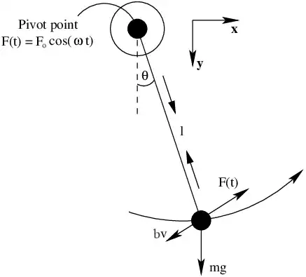
The resistive force has magnitude $bv$ and hence exerts a torque $-Lbv = -bL^2\dot{\theta}$.
The torque of the weight is $-mgL\sin\theta,$ and that of the driving force is $LF(t)$.
Thus, the equation of motion $I\ddot{\theta}=\Gamma$ is :
$\qquad mL^2\ddot{\theta} = -bL^2\dot{\theta} - mgL\sin\theta + LF(t) \tag{1}$
Assume that the driving force $F(t)$ is sinusoidal:
$\qquad F(t) = F_o\cos(\omega t) \tag{2}$
where $F_o$ is the drive amplitude (the amplitude of the driving force) and $\omega$ is the drive frequency.
Substituting $(2)$ into $(1),$ we find:
$\therefore \quad mL^2\ddot{\theta} = -bL^2\dot{\theta} - mgL\sin\theta + LF_o\cos(\omega t) \tag{3}$
or, $\qquad\ddot{\theta} + \frac{b}{m}\dot{\theta} + \frac{g}{L}\sin\theta = \frac{F_o}{mL}\cos\omega t \quad \left[ \because \ \frac{b}{m}=2\beta,\frac{g}{L}=\omega_o^2, \gamma=\frac{F_o}{mL\omega_o^2}=\frac{F_o}{mg} \right]$
Finally,
$\qquad\ddot{\theta} + 2\beta\dot{\theta} + \omega^2_o\sin{\theta} = \gamma\omega^2_o\cos\omega t \tag{4}$
where:
- Damping constant $= \beta ,$
- Natural frequency $= \omega_o ,$
- Driving strength $= \gamma$ (dimensionless).
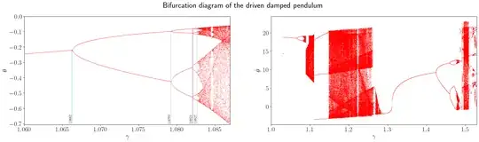
Bifurcation Diagram Plot
An algorithm based on your code for generating the bifurcation diagram of a DDP:
Algorithm: Bifurcation Diagram of a Driven Damped Pendulum
Initialize Parameters:
- Set the frequency of the driving force $\omega = 2\pi$.
- Set the natural frequency $\omega_o = 1.5 \times \omega$.
- Set the damping coefficient $\beta = \omega_o / 4$.
- Define the time step $\text{dt} = 0.01$.
- Define the time span $t_{\text{span}} = [0, 600]$.
- Set the initial conditions $x_0 = [-\pi/2, 0]$ for angle $\theta_0$ and angular velocity $\dot{\theta}_0$.
Define Sampling Points:
- Create a list of sampling points (indices) corresponding to times
from $t = 500$ to $t = 600 $ with a step size of $\text{dt}$.
Initialize Storage Arrays:
- Create empty lists
th and dth to store bifurcation data for $\theta$ and $\dot{\theta}$ respectively.
Loop Over Driving Force Amplitude for $\theta$ Bifurcation Diagram:
- For each value of $\gamma$ in a specified range $(e.g., \gamma \in [1.06, 1.087]):$
- Set the parameters $(\beta, \omega_o, \gamma, \omega)$.
- Solve the equation of motion using the RK4 method over the time span.
- Extract the $\theta$ values at the specified sampling points.
- For each sampled $\theta$, append the pair $(\gamma, \theta)$ to the list
th.
Loop Over Driving Force Amplitude for $\dot{\theta}$ Bifurcation Diagram:
- For each value of $\gamma$ in a specified range (e.g., $\gamma \in [1.03, 1.53]$):
- Set the parameters $(\beta, \omega_o, \gamma, \omega)$.
- Solve the equation of motion using the RK4 method over the time span.
- Extract the $\dot{\theta}$ values at the specified sampling points.
- For each sampled $\dot{\theta}$, append the pair $(\gamma, \dot{\theta})$ to the list
dth.
- Convert the lists
th and dth to arrays theta_bif and theta_dot_bif.
Plot Bifurcation Diagrams:
- Create a subplot with two plots:
- Plot $\gamma$ vs. $\theta$ using the data in
theta_bif.
- Plot $\gamma$ vs. $\dot{\theta}$ using the data in
theta_dot_bif.
- Label the axes and set appropriate limits for better visualization.