Scatter is indeed a big problem. We try to deduce whether detected photons are scattered by measuring their energy. With a modern PET detector, energy resolutions on the order of 12% FWHM (full width half maximum) are possible. This corresponds to a standard deviation of 26 keV, which means that you can reliably differentiate between photons that have energy of 511 keV, and those that have lost about 65 keV (2.5 standard deviations contains about 99%). A PET system will have a discriminator that makes sure the measured energy of the incoming photons falls within a certain range - sometimes called LLD (lower level discriminator) and ULD (upper level discriminator). The setting of the LLD in particular affects the scatter fraction that is admitted.
From the Compton scatter equation you find that a loss of 65 keV includes scatter angles up to about 31°:
$$E' = \frac{E}{1+\frac{E}{m_0 c^2}\left(1-\cos\theta\right)}\\
\cos\theta = 2 - \frac{E}{E'}$$
When photons undergo multiple scatters, they will lose even more energy. Bottom line is - a good fraction of scattered photons are eliminated by the energy discriminators, but a large number still get through. This means that scatter correction algorithms are a very important component of PET reconstruction algorithms. These cannot identify individual scattered photons that fell within the window, but they can attempt to estimate the average effect of scatter (which tends to add a low-frequency "blur" to the image - reducing both contrast and quantitative accuracy).
More importantly, there is a great deal of focus on improving the timing resolution of the PET detectors. Currently commercial PET detectors are produced with timing resolutions below 400 ps. Since PET events are detected in coincidence, this means that you can know the position of the annihilation along the line of response (LOR) within about 6 cm - not quite enough to put a dot in the image, but enough to help with the convergence of the reconstruction algorithm (in the process, this improves the SNR considerably). When events scatter, the place where they "apparently originated" will be off - this is something that needs to be corrected. But this is taken into account by the scatter correction algorithm.
As the count rate increases, the probability of two photons that did not originate from the same annihilation falling inside the same timing window increases quadratically - such an event is called a "random" event, and it can be very significant during the early parts of dynamic studies. At high enough activity, randoms dominate the event stream, and add so much noise to the image that the image quality degrades (even though the number of "good" events is increasing). This is traditionally measured using NECR - noise equivalent count rate - which is
$$\rm{NECR=\frac{T^2}{T+S+nR}}$$
Where $T$ = trues rate, $S$ = scatter rate, and $R$ = randoms rate. The value $n$ can be either 1 or 2, depending on how the correction for randoms is implemented. As you can see, if $\rm{R\propto T^2}$, that term will eventually dominate.
How much scatter is admitted into the PET ring is a strong function of geometry. In "the olden days", PET scanners used to have a set of thick tungsten septa: these would block radiation that didn't come from within a narrow range of angles. If an unscattered photon could make it through the septa, it was very likely that the other photon, after scatter, no longer "fitted" in the collimator. This made for a very effective scatter rejection. Unfortunately, the collimator also stopped a large number of "true" coincidences, and this reduced the overall sensitivity of the scanner. Today, no commercial vendor manufactures 2D scanners any more - the septa are gone, and scatter is corrected for algorithmically.
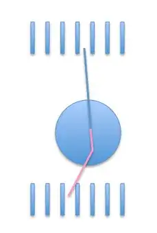
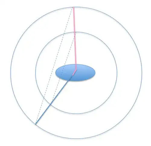
Even so, the geometry still matters. For example, for simultaneous PET/MR scanners, the diameter of the detector ring is small (the ring has to fit inside the MR). This means that many scattered photons end up with an apparent line of response "inside the object" - and that scatter fraction is therefore large. By contrast, when the ring is large, a scattered ray has a good chance of resulting in an apparent LOR that falls outside of the body - and therefore doesn't affect the image:
Incidentally - while the timing resolution can be below 400 ps, the "timing window" (that is, the difference in time of arrival that is considered acceptable) has to be larger than that, because when an event occurs near one of the detectors, the first photon will arrive much sooner than the second. For a field of view of 70 cm, this amounts to about 2.3 ns in each direction - so arrival times have to lie in a range of ±2.3 ns or so (there are some subtle interactions with timing resolution that I won't elaborate on).
Here is an example from this article on attenuation correction showing an image of a reconstructed PET whole body exam with attenuation and scatter correction applied (top row) and without (bottom row):
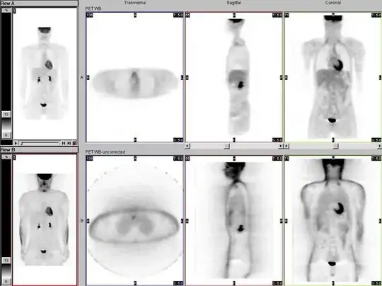
I believe the left-most image is a MIP (maximum intensity projection), while the next three are slices through the image volume: axial, sagittal, and coronal respectively.
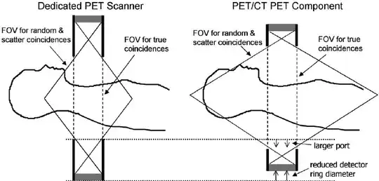
Two interesting things to note in the bottom row: first, the skin line is very "hot" - this is because there is less attenuation of photons traveling parallel to the skin, so during reconstruction these lines of response will be "over-represented". Second, without attenuation and scatter correction you see a lot of "fuzz" outside the body - this is the result of reconstructing "lines of scatter" that don't even intersect with the body (as you see also in my diagram above). Finally - you see a series of bands in the image. The PET scanner has an axial range of only about 15 cm, so to image a whole body you have to take multiple shots and stitch them together (usually done in a step-and-shoot fashion). At the end of the detector ring, they often place an "end shield" that extends beyond the detector - it effectively blocks radiation from outside the field of view. This results in less scatter in the "end slices" - so when you overlap views, the place where end slices overlap will have less scatter. This diagram from Alessio et al, 2004 shows what I am talking about:
Incidentally - among people who develop PET reconstruction algorithms for a living, it is considered that "scatter is job security". It's a really hard problem to solve properly - and although it keeps getting better, there's plenty left to do.


![By Dscraggs (Own work) [Public domain], via Wikimedia Commons](https://i.sstatic.net/yj8R6.png)