The core reason is that the chance for a given atom to decay in the next $n$ seconds is always the same.
You can get a more intuitive feel for this by considering a simple game with dice.
Start with some initial population of ordinary dice (I'll assume we're using the basic six-sided (cubical) ones, but you table top RPG fiends can use polyhedral ones if you want).
On each round roll all the surviving dice. Collect, count and remove any that show a 1; these are the ones that decayed and they are removed from the surviving population (they do not participate in future rounds). Record the number that decayed and the number that remain.
Continue with step #2 until none survive (or you get bored).
Repeat the whole of 1--3 several time to get some sense of the variation.
Graph both the (average) number that decay and the (average) number that survive as a function of the number of rounds. (For more insight, do this both on linear paper and on semi-log paper.)
You'll notice that the odd for any particular die to fail and be removed on any given round is always 1/6, which is equivalent to the constant odds for a unstable nucleus to decay in some give time frame.
You can also simulate this kind of experiment with a code like:
// Rolling dice radioactive decay demo simulator.
//
// During each round any die that rolls a 1 is removed from the
// population, and we plot the average number of dice surviving as a
// function of the number of rolls.
//
// Relies on the ROOT framework. http://root.cern.ch/
//
// Compile with
//
//    g++ -O3 $(root-config --cflags --ldflags --libs) decay.cc -o decay
//
// then run with
//
//     ./decay [<initial population> [<number of rolls> [<number of trials>]]]
//
// and find the output in "decay.png"
#include <iostream>

#include <TProfile.h>
#include <TCanvas.h>
#include <TRandom3.h>
#include <TF1.h>

int main(int argc, char*argv[]){

  // running parameters and default values
  int population = 1000;
  int timeticks = 25;
  int trials = 20;

  // trivial argument handling
  switch (argc) {
  default: /* FALL-THOUGH */
  case 4:  /* FALL-THOUGH */
    trials = std::atoi(argv[3]);
  case 3:  /* FALL-THOUGH */
    timeticks = std::atoi(argv[2]);
  case 2:  /* FALL-THOUGH */
    population = std::atoi(argv[1]);
  case 1:  /* FALL-THOUGH */
  case 0:
    break;
  }

  std::cout << "Doing " << trials
        << " trials of " << population
        << " dice over " << timeticks << " rolls."
        << std::endl;

  // Setup a profile histogram of the number of dice surviving at a
  // particular time over some number of trials
  TProfile*hS = new TProfile("hS","Surviving population",
                 timeticks+1,-0.5,timeticks+0.5);
  hS->GetXaxis()->SetTitle("Rolls");
  hS->GetYaxis()->SetTitle("Surviving dice");

  TProfile*hD = new TProfile("hD","Number decaying",
                 timeticks+1,-0.5,timeticks+0.5);
  hD->GetXaxis()->SetTitle("Rolls");
  hD->GetYaxis()->SetTitle("Decaying dice");

  // A PRNG
  TRandom*r=new TRandom3(0);

  for (int p=0; p<trials; ++p) { // Several passes to establish a profile
    if (p%5 == 0) std::cout << "   Trial " << p+1 << "..." <<std::endl;
    int count = population;
    int t=0;
    for (t=0; t<timeticks; t++) { // several time buckets to observe decay
      hS->Fill(t,count);
      int decay = 0;
      for (int i=count; i; --i) { // Try each surviving die
    if ( r->Integer(6) == 0) {
      --count; // discard this die if it rolls 1
      ++decay;
    }
      }
      hD->Fill(t,decay);
    }
    hS->Fill(t,count);
  }

  // Fit the data
  hS->Fit("expo","","",0.5,timeticks+0.5);
  hS->GetFunction("expo")->SetLineColor(kRed);
  hS->GetFunction("expo")->SetLineStyle(kDotted);

  hD->Fit("expo","","",0.5,timeticks+0.5);
  hD->GetFunction("expo")->SetLineColor(kBlue);
  hD->GetFunction("expo")->SetLineStyle(kDashDotted);

  // Output results
  TCanvas*c1 = new TCanvas("c1","c1",600,900);
  c1->Divide(1,2);
  c1->cd(1);
  hS->DrawCopy("");
  hD->DrawCopy("SAME");
  c1->cd(2);
  gPad->SetLogy();
  hS->Draw("");
  hD->Draw("SAME");
  c1->Print("decay.png");
}
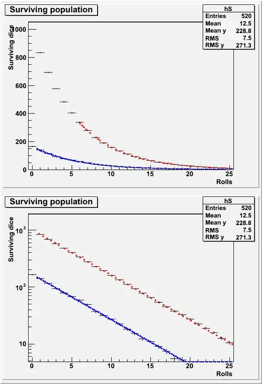
Using the default values (a great many dice for many trials of many rounds) you get something like
or with a number of dice, rounds and repeats that wouldn't bore a human to tears you get something like
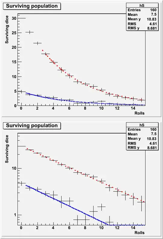
The fits are exponentials to show the functional dependence.