I use other symbols in order to prevent confusion in the following.
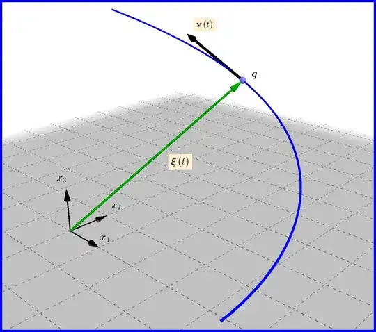
Let a point charge $\:q\:$ moving with position vector $\:\boldsymbol{\xi}\left(t\right)\:$ as in above Figure. Then the volume charge density and the charge current density are expressed via Dirac $\:\delta$-function as follows
\begin{align}
\rho\left(\mathbf{x},t\right) & =q\cdot\delta^{3}\bigl(\mathbf{x}-\boldsymbol{\xi}\left(t\right)\bigr)
\tag{01a}\\
\mathbf{j}\left(\mathbf{x},t\right) & =q\cdot\delta^{3}\bigl(\mathbf{x}-\boldsymbol{\xi}\left(t\right)\bigr)
\cdot\dfrac{d\boldsymbol{\xi}\left(t\right)}{dt}=q\cdot\delta^{3}\bigl(\mathbf{x}-\boldsymbol{\xi}\left(t\right)\bigr)\cdot\mathbf{v}\left(t\right)
\tag{01b}
\end{align}
where
\begin{equation}
\mathbf{v}\left(t\right)= \bigl(\upsilon_{1}\left(t\right),\upsilon_{2}\left(t\right),\upsilon_{3}\left(t\right)\bigr)= \biggl(\dfrac{d\xi_{1}\left(t\right)}{dt},\dfrac{d\xi_{2}\left(t\right)}{dt},\dfrac{d\xi_{3}\left(t\right)}{dt}\biggr)=
\dfrac{d\boldsymbol{\xi}\left(t\right)}{dt}
\tag{02}
\end{equation}
the velocity of the charge.
Under the assumption that the electric charge $\:q\:$ is invariant (observers in different inertial systems agree on the same value) we must show that the 4-quantity
\begin{equation}
\dfrac{\mathbb{J}}{q} \equiv \left[\delta^{3}\bigl(\mathbf{x}-\boldsymbol{\xi}\left(t\right)\bigr), \:\delta^{3}\bigl(\mathbf{x}-\boldsymbol{\xi}\left(t\right)\bigr)\cdot\dfrac{d\boldsymbol{\xi}\left(t\right)}{dt} \right]
\tag{03}
\end{equation}
is a 4-current. So we must prove that it satisfies the continuity equation
\begin{equation}
\dfrac{\partial \left[\delta^{3}\bigl(\mathbf{x}-\boldsymbol{\xi}\left(t\right)\bigr) \right]}{\partial t}+ \boldsymbol{\nabla}_{\mathbf{x}}\boldsymbol{\cdot} \left[\delta^{3}\bigl(\mathbf{x}-\boldsymbol{\xi}\left(t\right)\bigr)\cdot\dfrac{d\boldsymbol{\xi}\left(t\right)}{dt} \right]=0
\tag{04}
\end{equation}
or
\begin{equation}
\dfrac{\partial \left[\delta^{3}\bigl(\mathbf{x}-\boldsymbol{\xi}\left(t\right)\bigr) \right]}{\partial t}+ \boldsymbol{\nabla}_{\mathbf{x}}\boldsymbol{\cdot} \left[\delta^{3}\bigl(\mathbf{x}-\boldsymbol{\xi}\left(t\right)\bigr)\cdot\mathbf{v}\left(t\right)\right]=0
\tag{04a}
\end{equation}
If proved, this 4-current would be a 4-vector also.
Now
\begin{equation}
\delta^{3}\bigl(\mathbf{x}-\boldsymbol{\xi}\left(t\right)\bigr) =\delta\bigl(x_{1}-\xi_{1}\left(t\right)\bigr)\cdot\delta\bigl(x_{2}-\xi_{2}\left(t\right)\bigr)\cdot\delta\bigl(x_{3}-\xi_{3}\left(t\right)\bigr)
\tag{05}
\end{equation}
Using the following property of Dirac $\:\delta$-function
\begin{equation}
z\delta\left( z \right)=0 \Rightarrow \dfrac{\partial \delta\left(z\right)}{\partial z} = - \dfrac{ \delta\left(z\right)}{ z}
\tag{06}
\end{equation}
we have
\begin{equation}
\dfrac{\partial \left[\delta\bigl(x_{k}-\xi_{k}\left(t\right)\bigr) \right]}{\partial t}=\:+\:\dfrac {\dfrac{d \xi_{k}}{dt}}{x_{k}-\xi_{k}\left(t\right)}\cdot\delta\bigl(x_{k}-\xi_{k}\left(t\right)\bigr)=\:+\:\dfrac {v_{k}\left(t\right)}{x_{k}-\xi_{k}\left(t\right)}\cdot\delta\bigl(x_{k}-\xi_{k}\left(t\right)\bigr)
\tag{07}
\end{equation}
So
\begin{equation}
\dfrac{\partial \left[\delta^{3}\bigl(\mathbf{x}-\boldsymbol{\xi}\left(t\right)\bigr) \right]}{\partial t}=\:+\left(\sum_{k=1}^{k=3}\dfrac {v_{k}\left(t\right)}{x_{k}-\xi_{k}\left(t\right)}\right)\cdot\delta^{3}\bigl(\mathbf{x}-\boldsymbol{\xi}\left(t\right)\bigr)
\tag{08}
\end{equation}
On the same footing we can prove that
\begin{equation}
\dfrac{\partial \left[\delta\bigl(x_{k}-\xi_{k}\left(t\right)\bigr)\cdot v_{k}\left(t\right)\right]}{\partial x_{k}}=\:-\:\dfrac {v_{k}\left(t\right)}{x_{k}-\xi_{k}\left(t\right)}\cdot\delta\bigl(x_{k}-\xi_{k}\left(t\right)\bigr)
\tag{09}
\end{equation}
that is
\begin{equation}
\boldsymbol{\nabla}_{\mathbf{x}}\boldsymbol{\cdot} \left[\delta^{3}\bigl(\mathbf{x}-\boldsymbol{\xi}\left(t\right)\bigr)\cdot\mathbf{v}\left(t\right)\right]=\:-\left(\sum_{k=1}^{k=3}\dfrac {v_{k}\left(t\right)}{x_{k}-\xi_{k}\left(t\right)}\right)\cdot\delta^{3}\bigl(\mathbf{x}-\boldsymbol{\xi}\left(t\right)\bigr)
\tag{10}
\end{equation}
proving the continuity equation (04).
EDIT : A strange invariant
Realizing that the 4-quantity $\left(\mathbb{J} /\right)q$ of equation (03) is a contravariant 4-vector, say $\mathbb{V}$
\begin{equation}
\mathbb{V} \equiv \delta^{3}\bigl(\mathbf{x}-\boldsymbol{\xi}\left(t\right)\bigr)\cdot \left[c, \:\dfrac{d\boldsymbol{\xi}\left(t\right)}{dt} \right]=\delta^{3}\bigl(\mathbf{x}-\boldsymbol{\xi}\left(t\right)\bigr)\cdot\Biggl[\:\:c\:\:,\:\:\mathbf{v}\:\:\Biggr]
\tag{11}
\end{equation}
and having in mind- (and comparing it with-) the contravariant 4-vector for velocity
\begin{equation}
\mathbb{U} \equiv \gamma_{v}\cdot \left[c, \:\dfrac{d\boldsymbol{\xi}\left(t\right)}{dt} \right]=\gamma_{v}\cdot\Biggl[\:\:c\:\:,\:\:\mathbf{v}\:\:\Biggr]
\tag{12}
\end{equation}
I was wondering which would be the relation between the Dirac $\:\delta$-function $\delta^{3}\bigl(\mathbf{x}-\boldsymbol{\xi}\left(t\right)\bigr)$, a function of $\:\left(\mathbf{x},\:t\:\right)$, and $\:\gamma_{v}\:$, a function of $\:t\:$
\begin{equation}
\gamma_{v}= \left[1-\left(\dfrac{v}{c}\right)^{2}\right]^{-1/2}=\left[1-\left\Vert\dfrac{d\boldsymbol{\xi}\left(t\right)}{c dt}\right\Vert ^{2}\right]^{-1/2}
\tag{13}
\end{equation}
We know that the inner product of two 4-vectors (in Minkowski space) is Lorentz-invariant, so
\begin{equation}
\mathbb{U}\boldsymbol{\circ} \mathbb{V }= c^{2}\left[1-\left\Vert\dfrac{d\boldsymbol{\xi}\left(t\right)}{c dt}\right\Vert ^{2}\right]^{1/2}\cdot \delta^{3}\bigl(\mathbf{x}-\boldsymbol{\xi}\left(t\right)\bigr) = \text{invariant}
\tag{14}
\end{equation}
If we see this invariant in the rest frame of the particle, then
\begin{equation}
\bbox[#FFFF88,12px]{\left[1-\left\Vert\dfrac{d\boldsymbol{\xi}\left(t\right)}{c dt}\right\Vert ^{2}\right]^{1/2}\cdot \delta^{3}\bigl(\mathbf{x}-\boldsymbol{\xi}\left(t\right)\bigr) = \text{invariant}=\delta^{3}\bigl(\mathbf{x}_{rf}\bigr)}
\tag{15}
\end{equation}
where $\:\mathbf{x}_{rf}\:$ the position vector of a reference point with respect to the rest frame of the particle.
$=\!=\!=\!=\!=\!=\!=\!=\!=\!=\!=\!=\!=\!=\!=\!=\!=\!=\!=\!=\!=\!=\!=\!=\!=\!=\!=\!=\!=\!=\!=\!=\!=\!=\!=\!=\!=\!=\!=\!=\!$
$\:\color{red}{\textbf{THIS ANSWER OF MINE IS WRONG !!!}}$ because
Proofs that the 4-dimensional electric charge current density $\,\mathbf J\,$ is transformed as a Lorentz 4-vector based upon the conservation law (continuity equation) are false. That electric charge is constant in an inertial system doesn't provide any information about how it is transformed between inertial systems. It's a confusion between what is a constant (it concerns what happens in a system) and what is an invariant (it concerns what happens between two systems).
\begin{equation}
\partial_{\mu}A^{\mu}\boldsymbol{=}\texttt{invariant}\quad \boldsymbol{=\!\ne\!\Rightarrow}\quad A^{\mu}\boldsymbol{=}\texttt{contravariant Lorentz 4-vector} \tag{16}\label{16}
\end{equation}
