For a given Hamiltonian with spin interaction, say Ising model $$H=-J\sum_{i,j} s_i s_j$$ in which there are no external magnetic field. The Hamiltonian is invariant under transformation $s_i \rightarrow -s_i$, so there are always two spin states with exactly same energy.
For the magnetization $M = \sum_i s_i$, we can take the ensemble average $$\left\langle M\right\rangle =\sum_{\{s_{i}\}}M\exp(-\beta E)$$ and the result should be $\left\langle M\right\rangle = 0$ because the two states with all spin flipped will exactly cancel each other. There is an argument for this in the wiki.
So the question: how is this situation handled for finite and infinite lattice? How can they obtain the non-zero magnetization for the 2D Ising model?
$$M=\left(1-\left[\sinh\left(\log(1+\sqrt{2})\frac{T_{c}}{T}\right)\right]^{-4}\right)^{1/8}$$
Some information: for a 1D Ising model with external magnetic field, one can solve the Hamiltonian $$H=-J\sum_{i,j} s_i s_j - \mu B \sum_i s_i$$ and obtains the magnetization as $$\left\langle M\right\rangle =\frac{N\mu\sinh(\beta\mu B)}{\left[\exp(-4\beta J)+\sinh^{2}(\beta\mu B)\right]^{1/2}}$$ It gives the result $\left\langle M\right\rangle \rightarrow 0$ when $B \rightarrow 0$ for any temperature and this match the definition of the magnetization above. However, it gives $\left\langle M\right\rangle \rightarrow N\mu$ when we take the limit of $T \rightarrow 0$. It suggests the ordering of limit is important, but we still get $\left\langle M\right\rangle = 0$ when there is no external magnetic field.
Reminder: There are some precautions needed to care when you run computer simulation using the definition of magnetization above directly, otherwise, you will always get 0. These methods are similar to create a spontaneous symmetry breaking manually, for the Ising model, the following may be used:
- Use the $\left\langle |M|\right\rangle$ instead
- Fix the state of one spin so that the system will close to either $M=+1$ or $M=-1$ at low temperature.
In general, the finite size scaling should be used because we are likely interested in the thermodynamic limit of the system.
Update:
Visualization should explain the problem better. Here is the figure of the canonical distribution as a function of magnetization $M$ and temperature $T$ for 3D Ising model ($L = 10$).
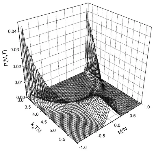
At a fixed temperature $T \lesssim T_c$, there are two symmetric peaks with opposite magnetization. If we blindly use the $\left\langle M\right\rangle$ defined before, we will get $\left\langle M\right\rangle = 0$. So how do we deal with this situation?
For a finite system, there is a finite probability that the transition between two peaks can occur. However, the "valley" between two peaks will become deeper and deeper when the size of the system $L$ increase. When $L \rightarrow \infty$, the transition probability tends to zero and those two configuration space should be separated. Note that the "flat mountain" in the figure at $L = 10$ will also become a very very sharp peak when $L \rightarrow \infty$.
One method discussed in the answers below is to consider the average of $M$ for separate configuration spaces. This seems reasonable for infinite system, but becomes a problem for finite system. Another problem raised here is that how to find each separated configuration spaces?
Thanks people try to give the answers to this question. In the following discussion, Kostya gives the typical treatment of spontaneous symmetry breaking. Marek discusses the ensemble average below and above the critical temperature. Greg Graviton gives an analogue for the real space spontaneous symmetry breaking.
If anyone can explain better to the problem of configuration space and how to take the average for Ising model, other spin models or general case, you are welcome to leave answer here.