Why is my Lyapunov exponent similar for single and double pendulum?

Question

This is my first question here on stackexchange. I hope that I can be understood. If not, tell me and I will reformulate and fill in with details.

I have simulated a single pendulum and a double pendulum in matlab to find the Lyapunov exponent. The single pendulum is a two dimensional system (angle $q$ and canonical momentum $p$) so there should be no chaos and no positive Lyapunov exponent. However, the Lyapunov exponent that I found was similar in magnitude compared to the double pendulum that I also simulated. The results are plotted in the figures below:

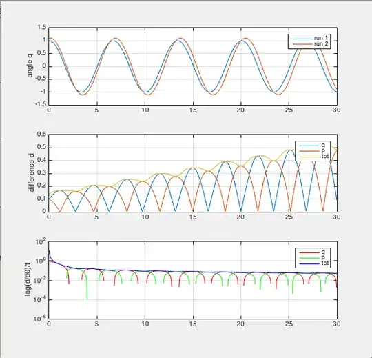
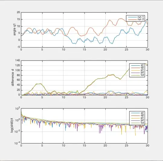
The first plot shows the time evolutions of the angle $q(t)$ for the pendulum arm. Both he simulations were run two times. The second run had initial conditions with all the coordinates displaced with the amount $d_0=0.1$.

The second plot shows the absolute value of the difference between the two trajectories as it evolves in time.

The third plot is the Lyapunov exponent which I derived from assuming that the separation between trajectories grows exponentially

\begin{equation} d(t)=|q(t)-q_e(t)|=d_0e^{\lambda t} \Rightarrow \lambda\left(t\right)=\frac{1}{t}\ln{\frac{d\left(t\right)}{d_{0}}} \end{equation} Where the subscript $e$ denotes the trajectory with the error in the initial condition.

The total separation between trajectories the double pendulum simulation is found with: \begin{equation} d_{tot}=\sqrt{(q_1-q_{1e})^2+(q_2-q_{2e})^2+(p_1-p_{1e})^2+(p_2-p_{2e})^2} \end{equation}

So why is the Lyapunov exponent for the two systems so similar? I thought the single pendulum would produce negative exponents and the double pendulum would produce an exponent in the magnitude of 10 to 20.

Answer 1

You are making to the following mistakes:

• Your initial displacement $d_0$ is 5 % of the variation of the respective variable, while it should be orders of magnitude lower. The Lyapunov exponent is defined for the limit of infinitesimal displacements, i.e., $d_0→0$.

• Your observation time is far too short. You are looking at four oscillations of your dynamics, when you could have thousands. The Lyapunov exponent is defined as the average over the whole attractor/trajectory.

• You do not consider multiple initial displacements or rescale the displacement vector. If you do not do this, the displacement will eventually grow to the size of the attractor and become meaningless.

In your specific example, the following happens:

• You seem to be using a pendulum without small-angle approximation and thus the frequency of your pendulum depends on the intial condition.

• Thus, your displaced system (red) has a slightly lower frequency than the original one and thus both systems dephase over time (at least that’s all they do in your short observation time). You see this as an increase of the distance which leads to your positive Lyapunov exponent.

• If you had used an infinitesimal excitation, the different frequencies would had little impact and you would have to be very precise to see them. For methods calculating the Lyapunov exponent in tangent space (e.g., Benettin et al.’s), this would have been no problem at all.

• If you had averaged over multiple initial displacements and, you would also have had displacements in which the phases would first align rather than diverge and I would intuitively say that on average you would have obtained a zero Lyapunov exponent (I cannot prove this though and it’s a rather meaningless excercise given the other mistakes).

I thought the single pendulum would produce negative exponents and the double pendulum would produce an exponent in the magnitude of 10 to 20.

The single pendulum should have a zero (largest) Lyapunov exponent like all limit cycle dynamics. You can understand this as follows: A displacement along the trajectory will neither shrink nor grow in time (on average). The two time series will be exactly the same except for an offset corresponding to the displacement.

I thought […] the double pendulum would produce an exponent in the magnitude of 10 to 20.

The absolute value of the Lyapunov exponent is rather meaningless, as it depends on how you scale time. Without knowing the detailed parameters of your double pendulum, it’s impossible to say what you should expect. The only thing that is meaningful is the sign of the largest Lyapunov exponent.

Answer 2

You will want to plot the exponent on a linear scale: the log scale is more appropriate for the difference graph should you choose to use it. The graphs for the exponent from differences in q and p individually may be misleading. You may also want to increase the time scale 100-fold so the phase space parameters of the single oscillators sync up a couple times. For the single oscillators without damping, the exponent should be 0 in the limit (check this chapter out). Otherwise, it looks like you should arrive at the right conclusion.