37

What kind of motion would a (preferably dimensionless for simplicity) body do if the force acted on it was proportional to the semi-derivative of displacement, i.e.

$$m \frac{\mathrm{d}^2 x}{\mathrm{d}t^2}=-k\frac{\mathrm{d}^{\frac12}x}{\mathrm{d}t^{\frac12}} \, \, ?$$

It would be helpful if someone with a copy of Mathematica plotted this for various values of the constants.

JamalS
  • 19,600
user148432
  • 515
  • 4
  • 11

6 Answers6

28

If $D^n$ denotes the $n$th derivative and $D^{-n}$ the $n$th integral, then we have that,

$$D^n f(t) = D^m[D^{-(m-n)}f(t)]$$

providing $m \geq \lceil{n}\rceil$. For our half derivative, we choose $n=1/2$, and $m=2$, in which case we have,

$$D^{1/2}f(t) = D^2[D^{-(3/2)}f(t)]$$

There is a general formula for the $n$th integral of a function, one of my favorite results of Cauchy:

$$f^{-(n)}(t) = \frac{1}{\Gamma(n)}\int_{0}^t (t-u)^{n-1}f(u) \, du$$

which is essentially a convolution $f(t) \ast t^{n-1}$. Applying it, we find,

$$D^{1/2}f(t) = \frac{d^2}{dt^2} \left[ \frac{2}{\sqrt{\pi}}\int_0^t (t-u)^{1/2}f(u) \, du\right]$$

Given the differential equation,

$$\frac{d^2 x(t)}{dt^2} = -\frac{k}{m} \frac{d^{1/2} x(t)}{dt^{1/2}}$$

we can substitute in our definition of $D^{1/2}x(t)$, and conclude,

$$x(t) = -\frac{2k}{m\sqrt{\pi}}\int_{0}^t (t-u)^{1/2}x(u)\, du + c_1t +c_2$$

for $c_1,c_2 \in \mathbb{R}$ which is an integral equation. If we can assume $x(t)$ is supported on $[0,\infty)$ only, then the integral is a convolution $x(t) \ast \sqrt{t}$ and taking the Laplace transform, we find,

$$X(s) = \left( 1+ \frac{k}{ms^{3/2}}\right)^{-1} \left( \frac{c_1}{s^2} + \frac{c_2}{s} \right) = \frac{m(c_1 + c_2 s)}{k\sqrt{s}+ms^2}$$

The solution $x(t)$ is then the inverse Laplace transform of $X(s)$. Formaly, this is given by,

$$x(t) = \frac{1}{2\pi i} \int_{\Gamma} e^{st} \frac{m(c_1 + c_2 s)}{k\sqrt{s}+ms^2} \, ds$$

where the contour $\Gamma$ is in the complex plane; it is a vertical line of infinite length with all poles of $F(s)$ to its left. In practice, we close the contour with an additional contour, ensure the second integral tends to zero (e.g. by the estimation lemma), and use the residue theorem.


The integrand, which we denote $F(s)$, has three poles located at $s^3 = k^2/m^2$, or equivalently,

$$s_1 = \omega^{4/3}_0, \quad s_2 = \frac{1}{2}(1+i\sqrt{3})\omega^{4/3}_0, \quad s_3 = \frac{1}{2}(i\sqrt{3}-1)\omega^{4/3}_0$$

as well as at $s_0= 0$, where we define $\omega^2_0 := k/m$. The vertical contour should begin after $s_1$ so all poles are to the left. However, doing so analytically is somewhat tedious. I chose to use a numerical method for the evaluation of inverse Laplace transforms due to H.E. Salzer which uses aquadrature formula. With Mathematica, I managed to reconstruct $x(t)$ partially:


enter image description here


in the simplified case when $c_1 = c_2 = k/m = 1$. It seems, by visual inspection, the solution resembles that of damped harmonic motion, such as when one introduces a damping term $\gamma \dot{x}$ in the equations of motion of a standard harmonic oscillator.

JamalS
  • 19,600
16

I am no mathematician and am a little afraid that my answer is too simple to be true, but here goes:

I use Fourier transforms to define the fractional derivative. $x(\omega)$ is defined such that

$$ x(t) = \int_{-\infty}^\infty \, \frac{\text{d}\omega}{2\pi} \text{e}^{i \omega t} \, x(\omega) \, .$$

Then any integer derivatives is

$$ \frac{\text{d}^n}{\text{d} t^n} x(t) = \int_{-\infty}^\infty \, \frac{\text{d}\omega}{2\pi} \text{e}^{i \omega t} \, (i \omega )^n \, x(\omega) \, ,$$

so that

$$ \left(\frac{\text{d}^n x}{\text{d} t^n}\right)(\omega) = (i \omega )^n \, x(\omega) \, .$$

Then this can be generalised to any real number $n$. In particular,

$$ \frac{\text{d}^{1/2}}{\text{d} t^{1/2}} x(t) = \int_{-\infty}^\infty \, \frac{\text{d}\omega}{2\pi} \text{e}^{i \omega t} \, \sqrt{i \omega } \, x(\omega) \, .$$

Since your equation is linear it can be solved separately for each Fourier modes. In Fourier space it becomes

$$ \left(- m \omega^2 + k \sqrt{i \omega}\right) x(\omega) = 0 \, .$$

This tells us that either $x(\omega) = 0$ or $ \omega^2 = \frac{k}{m} \sqrt{i \omega}$. The first solution is trivial. It is equivalent to $x(t)= 0$. The second however has four solutions:

\begin{align} & \omega_1 = \left(\frac{k}{m}\right)^{2/3} \text{e}^{i\,\pi/6} \, ,\\ & \omega_2 = \left(\frac{k}{m}\right)^{2/3} \text{e}^{i\,\pi/2} \, , \\ & \omega_3 = \left(\frac{k}{m}\right)^{2/3} \text{e}^{i \, 5\pi/6} \, , \\ & \omega_4 = 0 \, . \end{align}

Then the most general solution to your problem is

$$x(t) = C_1 \text{e}^{i\omega_1 t} + C_2 \text{e}^{i\omega_2 t} + C_3 \text{e}^{i\omega_3 t} + C_4\, .$$

$C_i$ are integration constants. Explicitly one finds,

$$x(t) = C_1 \, \text{e}^{i \,t \, (k/m)^{2/3} \sqrt{3}/2} \, \text{e}^{-(k/m)^{2/3} t/2} + C_2 \, \text{e}^{- (k/m)^{2/3} t} + C_3 \, \text{e}^{-i \, t \, (k/m)^{2/3} \sqrt{3}/2} \, \text{e}^{-(k/m)^{2/3} t/2} + C_4 \, .$$

We find three solutions that decay exponentially and one constant. Two of the decaying solutions oscillate as well.

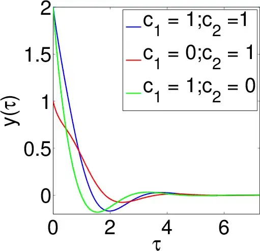
In order to make a plot, I set C_4 = 0 because this amounts to a simple vertical shift of $x(t)$, I choose $C_1 = C_2^* = (c_1 + i c_2)/2$ and $C_3 = C_3^*$ so that $x(t)$ is real, I rescale the time according to $\tau = t \, (k/m)^{2/3}/2$ and rescale $x(t)$ according to $y = x \, C_3$. Then my solution becomes,

$$y(\tau) = \text{e}^{-\tau} \left[ c_1 \, \cos(\sqrt{3} \, \tau) + c_2 \sin(\sqrt{3} \, \tau) \right] + \text{e}^{-2 \tau} \, .$$

Here is a plot of $y(\tau)$ for different values of $c_{1,2}$:

Plot of $y(\tau)$

8

You can simply take the semi-derivative of your equation again, which yields

$$\begin{align} m\frac{d^2}{dt^2}\underbrace{\frac{d^{\tfrac12}x}{dt^{\tfrac12}}}_{=-\frac mk\frac{d^2x}{dt^2}} &= -k\frac{dx}{dt} \\\Rightarrow m^2\frac{d^4x}{dt^4} &= k^2\frac{dx}{dt} \tag{*} \end{align}$$

and then solve that ODE. But, similarly to squaring an algebraic equation to eliminate roots, you (probably) have to discard halve of the solutions to satisfy the original equation.


As hinted at by user121330's comment, I assumed commutativity of $D^2$ (where $D:=d/dt$) and $D^{\tfrac12}$ which is not granted in general. I suspect that basically correlates with my above statement that some solutions of $(*)$ must actually be discarded. I'll try and think about this some more, but for now please be aware that there may be flaws or even uselessness in this answer...

4

One way to try to solve the equation is transforming it in an ODE. Apply the fractional derivative $D^{1/2}$ again to the equation to find $$D^{1/2}[D^2x(t)]=D^{5/2}x(t)-C_1t^{-3/2}-C_2t^{-5/2}-C_3t^{-7/2},$$ and $$D^{1/2}[D^{1/2}x(t)]=Dx(t)-C_4t^{-3/2}$$ Hence we got $$D^{5/2}x(t)=-\frac{k}{m}Dx(t)+C_1t^{-3/2}+C_2t^{-5/2}+C_3t^{-7/2}$$ But, we also have that $$D^{5/2}x(t)=D^2[D^{1/2}x(t)]=-\frac{m}{k}D^4x(t)$$ Hence we get the following ODE: $$x^{(4)}(t)-\omega^3 x'(t)=C_1t^{-3/2}+C_2t^{-5/2}+C_3t^{-7/2},$$ where $\omega^3=\dfrac{k^2}{m^2}$ Let $x'(t)=v(t)$ to get $$v'''(t)-\omega^3 v(t)=C_1t^{-3/2}+C_2t^{-5/2}+C_3t^{-7/2}$$ The general solution of the homogeneous equation for $v(t)$ is $$v_0(t)=c_1 e^{\omega t}+e^{-\omega t/2}\left(c_2\cos\dfrac{\sqrt3}{2}\omega t+c_3\sin\dfrac{\sqrt3}{2}\omega t\right)$$ The general solution of the homogeneous equation $x(t)$ is then $$x_0(t)=c_1 e^{\omega t}+e^{-\omega t/2}\left(c_2\cos\dfrac{\sqrt3}{2}\omega t+c_3\sin\dfrac{\sqrt3}{2}\omega t\right)+c_4,$$ where the constants are different in the two last equations. So, the general solution is of the form $$x(t)=x_0(t)+x_p(t),$$ where $x_p(t)$ is the particular solution.

3

An attempt for a more explicit solution. Using the definition of the half-derivative given by JamalS, one can transform the differential equation using the Laplace transform and get $$s^2X(s)-sx(0)-x'(0)=-\gamma^3{\sqrt s}\;X(s)$$ where $\gamma=\sqrt[3]{\frac km}$ is a positive constant. Solving for $X$ gives $$X(s)=\frac{sx(0)+\dot x(0)}{s^2+\gamma^3{\sqrt s}}.$$ Let us call $G(s)=1/(s^{3}+\gamma^3)$. The Laplace inverse of $s^{-1/2}G(s^{1/2})$ is given by (Erdelyi, Table of integral transforms, chapter IV, equation 4.1.33) $$z(t)=\frac{1}{\sqrt{\pi t}}\int_0^\infty g(u)\mathrm e^{-u^2/4t}\mathrm du.$$ Therefore we have $x(t)=\dot x(0)z(t)+x(0)\dot z(t)$.

Computation of $z(t)$ Let us write $\mathrm j=\mathrm e^{\mathrm i 2\pi/3}$. The inverse $g(t)$ of $G(s)$ is a simple Laplace inversion and yields $$ g(t)=\frac1{3\gamma^2}\left[\mathrm e^{-\gamma t}+\mathrm e^{-\mathrm j\gamma t}+\mathrm e^{-\mathrm j^2\gamma t}\right]$$ Let us now write $$\Phi(a,t)=\frac{1}{\sqrt{\pi t}}\int_0^\infty\mathrm e^{-a u}\mathrm e^{-u^2/(4 t)}\mathrm du=\mathrm e^{a^2 t}\mathrm{erfc}(a\sqrt t)=\varphi(a^2t).$$

EDIT

A remarkable property of $\varphi$ is $\varphi'(x)=\varphi(x)-\frac1{\sqrt{\pi x}}$. Reporting in the definition of $z$ we find $$z(t)=\frac1{3\gamma^2}\left[\varphi(\gamma^2 t)+\varphi(\mathrm j\gamma^2t)+\varphi(\mathrm j^2\gamma^2 t)\right].$$ $$ \dot z(t)=\frac13\left[\varphi(\gamma^2 t)+\mathrm j\varphi(\mathrm j\gamma^2 t)+\mathrm j^2\varphi(\mathrm j^2\gamma^2t)\right]-\frac2{3\sqrt{\pi\gamma^2t}}$$

Mathematica made the following plots of $z(t)$ and $\dot z(t)$ for $\gamma=1$, showing that $z$ is quite severely damped.

enter image description here

Tom-Tom
  • 1,989
3

So, what you have here is, as others have mentioned, a fractional order differential equation. Since others have provided graphs, there seems to be little point to adding one. Also, you seem more interested in the qualitative aspect than actual analytical solutions, as you've mentioned.

In essence, what you have here is some second order system with some element that behaves like something between a spring and a damper. There is some dissipative behavior that will come into play here, but also some oscillatory behavior, as you see from the other graphs.

A special result of this being a fractional order system is that that specific derivative is also non-local, meaning that the current dynamics of the system are not only dependent on the current state, but also past state. This is called historicity, or a system with memory.

There are many ways to represent that fractional order derivative mathematically, if you want to get into that. Most of the people here seem to have used some integral definition (whether explicitly, or in the case of the Laplace transform, implicitly), but you can also represent it as a series.

If you wanted a full on analytical solution, you might run into some non-elementary functions, but you can derive series representations from them using some of the methods that Odibat as developed as a result of his work on generalized Taylor series expansions.

If you have any more questions, let me know.

Ron
  • 421