The key to understanding image generation in MRI lies in realizing that the signal sent to the antenna (or coil) by the patient's tissues includes two different types of information:
- Information regarding the magnitude of the transverse magnetization of the tissue under the influence of a structured sequence of RF stimulation pulses. This magnitude depends on the tissue composition of every single voxel (3D pixel) of the anatomy being interrogated, and will be coded for medical interpretation by mapping it to gray-scale values to generate the final image.
- The necessary spatial encoding that will allow tracing back each component of the signal to a specific location in physical space.
In the following diagram of an MRI of the brain in progress, two voxels (red and magenta) are highlighted, and their individual signals added up to form a resultant wave, filling in a line in k-space (Fourier space):
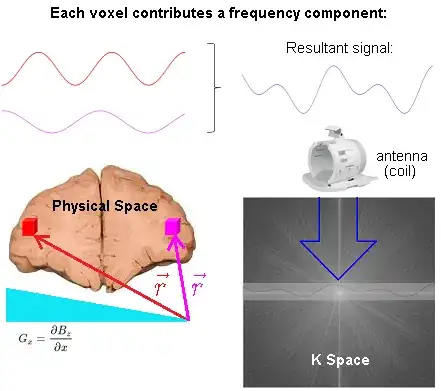
The spatial information is induced via linear gradient fields. At any particular point in space, i.e. $\color{red}{\vec r}$ corresponding to the location of the red voxel, the precession frequency of the atoms of hydrogen is (rotating frame):
$$\omega =\gamma\, \vec G_z \cdot \color{red}{\vec r}$$
with $\gamma$ corresponding to the gyromagnetic ratio; and $\vec G_z,$ the 3D gradient of the magnetic field $\vec G_z = \nabla B_z.$
The phase of the hydrogen atoms at location $\color{red}{\vec r},$ is the time integral of
$$\begin{align}
\phi(\color{red}{\vec r}, t) &= \int_0^t \omega(\color{red}{\vec r},\tau)\,\mathrm d\tau\\
&=\int_0^t \gamma\, \vec G_z(\tau) \cdot \color{red}{\vec r} \, \mathrm d\tau \\
&= \left( \gamma \int_0^t \vec G_z(\tau) \, \mathrm d\tau \right) \cdot \color{red}{\vec r} \\
&= \vec k(t) \cdot \color{red}{\vec r}
\end{align}$$
where $\vec k(t)=\gamma \, \int_0^t \vec G_z(\tau)\, \mathrm d\tau$ is defined such that it parametrically describes a path through spatial frequency space.
The signal acquired in MRI is the sum of all transverse magnetization:
$$\begin{align}
\color{purple}{\text{Signal}}(t) & \sim \int_{-\infty}^\infty M_{xy}(\vec r, t)\,\mathrm dx\mathrm dy\mathrm dz\\[2ex]
&=\int_{-\infty}^\infty M_{xy}(\vec r,t)\, \mathrm d\vec r \\[2ex]
& = \large \int_{-\infty}^\infty \underbrace{M_{xy}(\vec r, t=0)}_{\color{blue}{\text {Image}}} \, \underbrace{\mathrm e^{-\mathrm 2\pi i \,\vec k(t) \,\cdot\, \vec r}}_{\color{orange}{\text{Phase rotation}}} \mathrm d\vec r \tag 1
\end{align}$$
The phase rotation depends on time and space and does not affect the magnitude of the magnetization (or signal).
Equation $(1)$ is a Fourier transform relating $\color{purple}{\text{Signal}}$ as a function of time and the $\color{blue}{\text {Image}}.$
Decomposing equation $(1)$:
$$\text{Slice signal}_{k_x,k_y}=\int_{\text{slice}}\int_{\text{slice}}\rho_{(x,y)}\rm e^{-2\pi i \color{blue}{k_x} x} \;\rm e^{-2\pi i \color{red}{K_y} y}\rm dx \rm dy\tag 2$$
where $\color{blue}{\small \text K_x = \frac{\gamma}{2\pi}G_x \times t}$ and $\color{red}{\small \text K_y = \frac{\gamma}{2\pi}G_y \times \tau_{pe}},$ in which $\tau$ is the time for which the phase encoding gradient is applied, $\rho_{(x,y)}$ are the characteristics of the tissue in the anatomy we are trying to image, and $\gamma$ is the gyromagnetic ratio. This expression clearly relates the variable time in the read-out gradient with the values of the complex sinusoids obtained by integrating at each point in time over the entire slice.
Each point in physical space (patient) will contribute one frequency component to the time domain signal. Conversely, each point in k-space represents the magnitude of one given spatial frequency over the whole image.
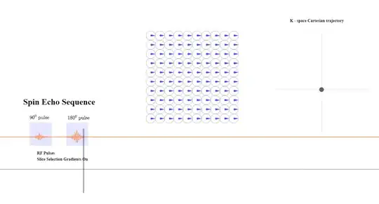
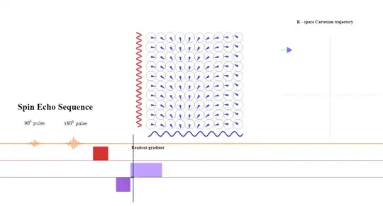
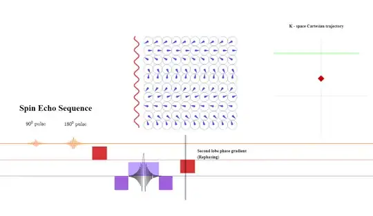
Critically, there is no FFT between signal reception ("Resultant signal" captured by the antenna (coil) in the diagram above) and the line in K-space being filled in. The signal received is already in Fourier space thanks to the action of the gradients that induce different spatial frequencies across the $x$- and $y$-axes in real space. Here is the diagrammatic depiction (inspired by this great animation by Tyler Moore on youtube) of the resulting phase differences induced by the application the phase and frequency encoding gradients used to obtain a line of K-space in a spin echo sequence ($*$ applicable to turbo spin echo - see below for explanation of turbo spin echo):
Initially, the slice selection gradient is turned on during the application of the $90^\circ$ (excitation) and $180^\circ$ (refocusing) pulses. There is no travelling in k-space yet:
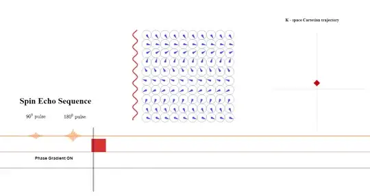
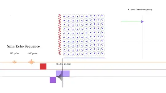
In the next step, the phase-encoding gradient is turned on: the gradient strength or amplitude as well as the time during which the gradient is applied determine the distance away from the $x$-axis the line about to be read will be in k-space because of the equation $\color{red}{\small \text K_y = \frac{\gamma}{2\pi}G_y \times \tau_{pe}}$ above $(2)$ (this is schematized as a red diamond travelling up along the $y$-axis in k-space while the phase gradient is on):
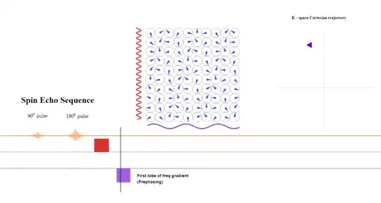
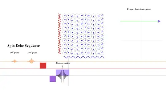
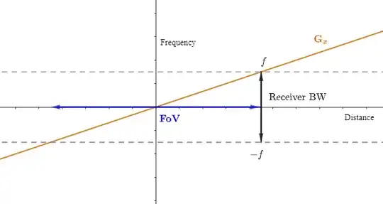
A pre-phasing lobe of the frequency-direction gradient will be turned on right after the phase-encoding gradient is applied. The amplitude or intensity of the gradient will determine the bandwidth of frequencies (given a fixed FoV). The longer it is applied, the more dephasing between anatomical points along the $x$-axis (frequency). During the application of the pre-phasing lobe, the position along k-space will become negative getting ready for the acquisition of a line of from left to right (purple arrowhead pointing left):
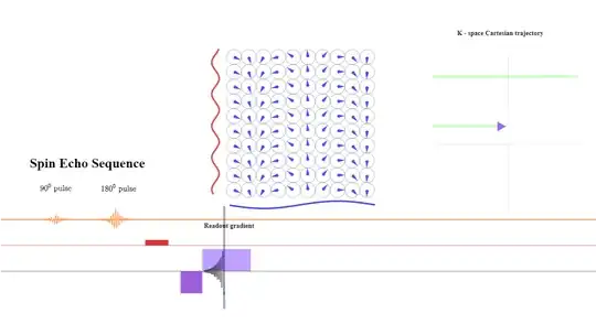
At the beginning of the read-out gradient, the first data point collected corresponds to the maximum negative value of $\color{blue}{\small \text K_x = \frac{\gamma}{2\pi}G_x \times t}$ due to the negative prephasing (or dephasing lobe) shown above, the second data point to a slightly more positive value of $\small \text k_x$ (arrowhead pointing right):
At the $\text {TE}$ point the spins still subject the same gradient amplitude (although reverse sign to the prephasing gradient) will have had a chance to revert the initial dephasing effect caused by the initial negative frequency prephasing gradient, showning no residual dephasing in the frequency direction - at that point only the effect exerted by the initial phase gradient will be apparent. The signal returned to the antenna will have maximum intensity:
During the second half of the read-out gradient dephasing in the opposite direction will increase over time and cause loss of signal strength in a mirror-like fashion that can be harnessed to save acquisition time. In practice, more than $50\%$ of the echo is sampled, but not all of it is needed. In partial-echo techniques it is the last part of the signal that is sampled to decrease the TE by shortening the readout gradient.
After the line of k-space is completed, a negative lobe in the frequency direction will be again applied to rephase the spins:
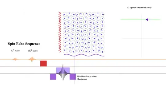
The dephasing along the phase initially introduced will be now reverted to return to the center of k-space:
After that, the process will be repeated to obtain another line of k-space (within the same TR in TSE, or in a different TR in classic spin-echo) (second green line in k-space below). The order in which k-space will be filled-in is not random, but rather follows a strategy (for instance 'linear' in which the center of k-space ($\text k_0$ or "contrast line" is acquired in the middle of the read-out; or 'low-high', in which the contrast line is acquired first, followed by more peripheral lines):
There is a need for as many phase encoding steps as the matrix in the phase encoding direction. The explanation is that when two constituent sinusoids contributing to the signal emitted by the patient have the same frequency, and vary only in phase, they cannot be distinguished (see here).
I have tried to reproduce the process of filling k-space in this applet, illustrating a single-echo SE acquisition.
In Eq $(2)$ the signal is expressed as a function of each coordinate in k-space, which in turn depends on the readout time $t$ and the phase gradient applied $\tau_{pe}.$ Going back to $\color{blue}{\small \text K_x = \frac{\gamma}{2\pi}G_x \times t}$ the strength of the gradient will remain unchanged during the acquisition of a line of k-space, and therefore will the difference in precession frequency between adjacent points in the anatomy in the frequency direction, or the actual frequency at each anatomical point. During the read-out all the frequencies from each anatomical point within the slice are sampled and digitized by the ADC (see below) to produce a point in k space.
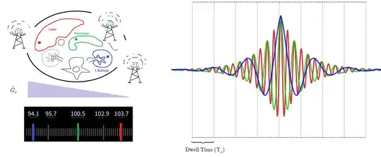
A true-to-fact visualization of the process can be as follows: Consider three tissue cells anatomically separate in the body. The red cell is part of the liver and happens to lie at one end of the gradient (for simplicity, just the frequency gradient $\vec G_x$) with its hydrogen atoms precessing at a frequency much higher than a blue cell in the left kidney (opposite side of the belly), which spins are slowest. In between an orange cell in the pancreas will precess at an intermediate frequency. Essentially, and throughout the emission of the signal back from the patient, these three cells will act as radio stations on the FM dial, emitting at a fixed frequencies. The intensity of the signal for each one of these three cells will increase progressively to the middle of the echo without changing their individual frequency, only to decrease progressively after that point in a symmetrical fashion.
The ADC (see below) will listen to the sum of all the frequencies coming back from the slice (red, orange and blue) at the same time in each digitization sample, collected at regular intervals (dwell time) (see below). Each sample will be directly allocated to the proper position on k-space according to complex plane coordinates, and only at a later point a FFT (or wavelet transform) will generate the final image.
Given that the integral of frequency over time is the definition of phase, it will actually be the dephasing along the phase and frequency directions induced by the gradients that will produce the signal. This is more clearly apparent in the expression on page 41 of Richard Ansorge's The Physics and Mathematics of MRI, in which the signal becomes a function solely of time:
$$\begin{align}
S(t)&=\int\int\int_{\text{FoV}} \rho(\vec r)\; \mathrm e^{-\mathrm i \omega_0 - \mathrm i \theta_{\text{acc}}}\mathrm dx\mathrm dy \mathrm dz\\[2ex]
&= \mathrm e^{-\mathrm i \omega_0 t } \int\int\int_{\text{FoV}} \rho(\vec r)\; \mathrm e^{-\mathrm i 2\pi \vec k \cdot \vec r}\mathrm dx\mathrm dy \mathrm dz
\end{align}$$
The effect of a particular gradient is to cause a local additional instantaneous precession $\gamma_p {\bf\vec G}(t) \cdot \bf \vec r,$ thus if the transverse spins were in phase at some time $t_0$ (say due to a $90^\circ$ RF pulse) than at a later time, $t,$ the accumulated phase offset $\phi_{\text{acc}}(\bf\vec r,t)$ is given by
$$\theta_{\text{acc}}({\bf \vec r}, t)= \gamma_p \Bigg[\color{orange}{\int_{t_0}^t \vec {\bf G}(\tau)\mathrm d\tau} \Bigg]\cdot \bf \vec r= 2\pi \;\color{orange}{\bf\vec k} \cdot \bf \vec r;$$
where $\rho(\vec r)$ is the proton density in different locations; and $\omega_0$ is the Larmor frequency induced by the main magnetic field $B_0.$
The amplitude and phase of the signal will be treated as real and imaginary components in the receiver. The ADC transforms the analog to digital signal:
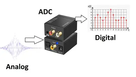
The ADC rating depends on the sample rate or sampling frequency (how closely the samples can be taken) and the amplitude or resolution (for example 16 or 24 bits). The actual process calls for a preamplification and a demodulation of the Larmor carrier frequency $(\small 50–300 \text{MHz})$ to be able to capture the information in the MR signal contained within a small bandwidth $\small \leq 1–2 \text{ MHz}),$ determined by the maximum gradient strength and the field of view (FOV), before the ADC conversion.
At this point in the process a filter (cosine, cosine squared, Fermi,
Gaussian, Hamming, Lorentzian, Riesz, Tukey,or others) operating in k-space will be applied to remove salt-and-pepper noise (SPN) occurring during the process of acquisition and transmission.
The spacing between samples is referred to as the dwell time (time between digitized samples), whereas the reciprocal of the dwell time $\small (\text{T}_s=\Delta t)$ is the sampling bandwidth $\small (\text{RBW}=1/\Delta t),$ or sampling rate $(\text f_s).$
The sampling bandwidth and the number of sampled points (matrix size in the frequency direction) determine the sampling time: $\small \text{Total sampling time} =\text{Matrix}_{\text{fr.}} \times \frac{1}{\text{RBw}} =\text{Matrix}_{\text{fr.}} \times \text{Dwell time}.$
Each frequency can be sampled by the receiver for a shorter or longer period of time, and the longer each frequency represented in k-space is sampled (lower bandwidth), the higher the signal-to-noise (SNR)$(**)$ will be, at the cost of a slower readout rate.
An ADC effectively averages the input signal over the dwell time, thus the effective noise on the digitized signal is proportional to $\small 1/\sqrt{\Delta t}$ making it desirable to increase $\small \Delta t.$ Signal noise [sic] is also directly proportional to the receiver bandwidth. Richard Ansorge and Martin Graves - The Physics and Mathematics of MRI.
A higher bandwidth results in reductions in the minimum $\small \text{TR}$ and $\small \text{TE},$ potentially decreasing scan time (provided the contrast afforded by minimal $\small \text{TR}$ values are medically desirable). A higher receiver bandwidth will sample more points per msec at the expense of lower SNR (see here), but with the upside of obtaining more closely packed echoes (shorter echo spacing, ESP), allowing a longer ETL's for a given $\small\text{TR}$: $\small \text{ESP}\sim \frac{\text{freq encoding steps}}{\text{sampling bandwidth}}.$ Reducing the acquisition time by increasing the bandwidth is not typically done, although there are some exceptions, such as 3D gradient (FFE) sequences here: although a higher bandwidth will decrease the sampling time, it is going to make a difference only as long as it allows a shorter minimum $\small \text{TR},$ and that lower $\small \text{TR}$ is desirable to achieve the contrast in the image intended - otherwise the few milliseconds saved are not comparable to the $\small \text{TR}.$
From a different perspective, the receiver bandwidth is defined as $\small \text{BW} =\text f_s \times \text{Matrix}_{\text{fr}}=\text f_s \times \text{No. samples}.$ This definition is different from the one above (sampling rate). There is a third concept of bandwidth as the range of precession frequencies that need be included for a chosen FoV:
$$\text{rBW (range of freq)}= \frac{\gamma}{2\pi} \times\text G_x \times \text{FoV} $$
Both expressions will match: sampling at the Nyquist rate, and given a matrix or number of points to sample, $\small \text{T}_s=\text{Pixels (no. sampled points)} / (2\times \text{max freq}).$
The gradient steepness and the bandwidth will have to move in synch unless the FoV is to be changed. On the other hand, if a change of FoV is introduced by the operator, the MRI unit will first try to achieve the desired FoV by changing the gradient. Only if changing the gradient is not enough to achieve the target FoV at a given matrix due to engineering limits, will the rBW be altered. The reason for this hierarchy of tasks is that changing the rBW will also alter the SNR or introduce chemical shift.
$(*)$ In a turbo spin echo (TSE) (same as fast spin echo (FSE)) each excitation pulse (90-degree pulse) is followed by a series of equally-spaced refocusing 180-degree pulses (echo-train length or ETL) and a corresponding echo will be collected after each of these refocusing pulses. This is just a strategy to save time by extracting several echoes out of every excitation pulse instead of the single-echo scheme of a conventional SE. From The Physics and Mathematics of MRI a CSE sequence would be of the form:
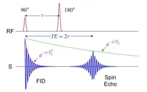
The refocusing $\small 180^\circ$ pulse is meant to re-phase the spins, causing them to regain coherence and thereby to recover transverse magnetization, which is really what is being captured. The $T_2^*$ of free-induction decay (FID) (see illustration above) is thus modified into a less rapid decay. The $\small 180^\circ$-pulse is half-way between the $\small 90^\circ$ pulse and the echo.
On a FSE sequence the diagram is:
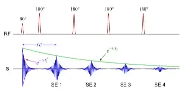
The acquisition time that would be calculated in conventional spin echo (CSE) as $\small\text{TR} \times \text{no. phase encoding steps N}_y \times \text{no. of averages (NEX)}$ indicating that to fill in k-space the number of different excitation pulses necessary is now reduced by a factor of ETL:
$$\text{Acquisition time}=\frac{ \text{TR} \times \text{matrix (Ph.)} \times \text{NEX}\times \text{no. packages}}{\text{ETL}\times \text{SENSE accel.}}\tag 3$$
The concept of package is explained below. SENSE (and compressed SENSE) are not explained.
Clinical MR exams are obtained as a set of stacks of images through the anatomy of interest at different desired planes and angulations and with different types of contrast between normal and diseased tissues and organs (e.g. T1, T2, proton density (PD)) $(***)$. Each of these stacks of images have identical parameters, and are called sequences.
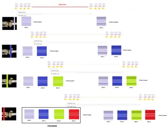
Typically, the slices or images in a given sequence will be obtained in packages (interleaved) - approximately $5$ or $6$ for a $\text{T}1$-weighted sequence and $2$ or $3$ for a $\text{T}2$ or $\text{PD}$ sequence. This takes advantage of the dead time imposed by the $\text{TR}$ or time between $\small 90^\circ \text{ pulses}.$ For example, if the $\text{TE}$ is $80$ msec, and the $\text{TR}$ $3,000$ msec, depending on the echo train there may be some $2,900$ msec of dead time, which can be used to consecutively select other slices (slice selection gradient) and proceed with the sequence of $\small 90^\circ$ excitation pulse, followed by the corresponding train of $\small 180^\circ$ pulses in as many slices as can be fit in this otherwise idle time interval. Within each of these packages or $\text{TR}$-sets each of the slices included will have a number of lines of k-space recorded equal to the echo train length. Importantly, these slices are not consecutive to avoid crosstalk. In a $2$-package sequence, the slices will be separate by one: $\{1,3,5, \dots\}$ for package $1$ and $\{2,4,6, \dots\}$ for package $2.$ For a $3$-package sequence, $2$ anatomically consecutive slices will be skipped.
The sequence of events is: With the slice selection gradient on, a $\small 90^\circ \text{ pulse}$ for the first slice in a package starts the "timer" for the repetition time $\small \text{TR}.$ This is followed by a train of $\small 180^\circ$ refocusing pulses and corresponding echo collection to fill a number of lines in k-space equal to the train length for the first image in the package. Then the same happens for the second image (anatomically separate) and so forth and so on until the last image in the package. At that point the "timer" for the $\small\text{TR}$ stops as a new $\small 90^\circ \text{ pulse}$ is emitted to selectively excite slice the first image all over again to obtain a new number of lines equal to the train length to continue filling k-space for as many lines as the matrix in the phase direction dictates. Hence $\small\text{TR}$ is the distance between two consecutive $\small 90^\circ$ pulses, and in every $\small \text{TR}$ a number of lines equal to the train length will be added to k-space for each of the images contained in the same package.
The need to selectively excite each of the slices and sample the corresponding echoes in the train limits how short the $\small \text{TR}$ can be set by the MRI unit. A separate issue limiting how short the $\small \text{TR}$ can go to save time is the SAR (Specific Absorption Rate) leading to tissue heating.
$(**)$ The SNR doesn't solely depend on the bandwidth. In fact, the SNR is controlled by
$$\small \text{SNR} \sim \text{VS} \times \sqrt{\frac{\text{No. Phase steps (Matrix)}\times\text{ No. Averages (NEX)}}{\text{rBW} } }\tag 4$$
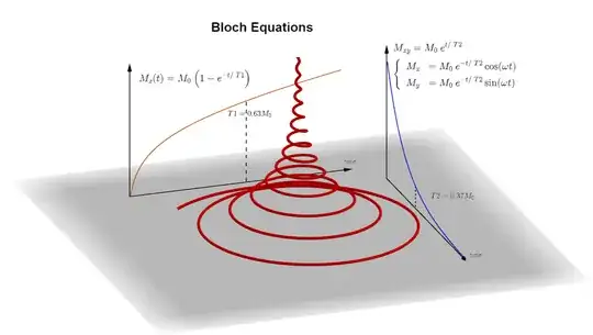
$(***)$ The signal is generated by the transverse tipping of the hydrogen spins. The transverse magnetization decays over time as the longitudinal magnetization along $B_0$ recovers, as encapsulated in the Bloch equations:
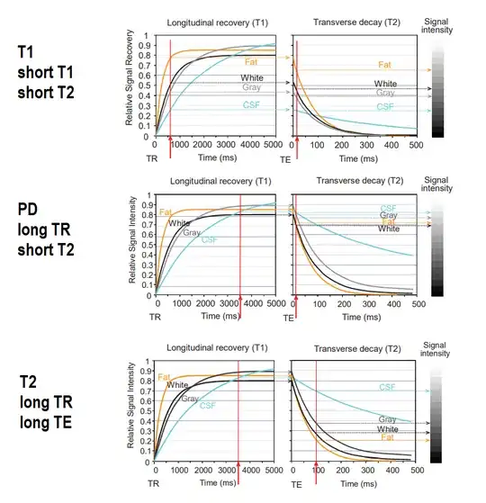
Different normal and pathologic tissues differ in $\small \text T1, \; \text T2$ or concentration of hydrogen atoms (proton density or $\small \text{PD}).$ This is exploited to obtain different types of diagnostic contrast on the MRI images. To do so the repetition and echo times are adjusted to capture maximal differences (from here):
Resources:
A K-space analysis of Small-Tip-Angle-Excitation by John Pauly et al. JMR 1989
MRI: Introduction to K-space by Eric Wong
Fast Spin Echo - Spaces Animation by Tyler Moore
The Physics and Mathematics of MRI by Richard Ansonge and Michael Graves
MRI Physics: MRI Image Formation Parameters, SNR, and Artifacts


