In the method below all the portfolio values at each time interval are calculated. Then they are aggregated in each time period and the period return is calculated. Finally the period returns are compounded and annualised.
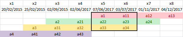
For example, the portfolio return between periods x5 and x6 is
(a11 + a23 + a34)/(a1 + a22 + a33) - 1 = 0.903 %
where a1 is the starting value of asset 1 and a11 is the value of asset 1 after one time period. If the actual values were known this would give a better result, but given the limited information they are calculated.
Compounding the period returns is the same as taking the time-weighted return.
s1 = {2017, 6, 7};
e1 = {2017, 12, 4};
s2 = {2015, 9, 2};
e2 = {2017, 11, 1};
s3 = {2015, 2, 25};
e3 = {2017, 7, 3};
s4 = {2015, 2, 20};
e4 = {2017, 6, 2};
d1 = QuantityMagnitude@DateDifference[s1, e1, "Day"];
d2 = QuantityMagnitude@DateDifference[s2, e2, "Day"];
d3 = QuantityMagnitude@DateDifference[s3, e3, "Day"];
d4 = QuantityMagnitude@DateDifference[s4, e4, "Day"];
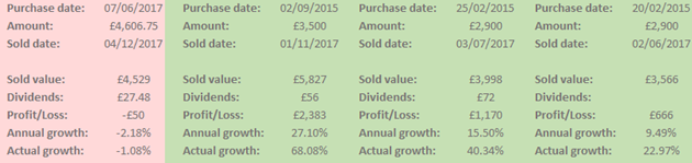
a1 = 4606.75;
v1 = 4529 + 27.48;
a2 = 3500;
v2 = 5827 + 56;
a3 = 2900;
v3 = 3998 + 72;
a4 = 2900;
v4 = 3566;
r1 = (v1/a1)^(1/d1) - 1.0
r2 = (v2/a2)^(1/d2) - 1.0
r3 = (v3/a3)^(1/d3) - 1.0
r4 = (v4/a4)^(1/d4) - 1.0
-0.0000609549
0.000656731
0.000394644
0.000248211
The above are the daily rates of return for the four assets.
x1 = {2015, 2, 20};
x2 = {2015, 2, 25};
x3 = {2015, 9, 2};
x4 = {2017, 6, 2};
x5 = {2017, 6, 7};
x6 = {2017, 7, 3};
x7 = {2017, 11, 1};
x8 = {2017, 12, 4};

k1 = QuantityMagnitude@DateDifference[x1, x2, "Day"];
k2 = QuantityMagnitude@DateDifference[x2, x3, "Day"];
k3 = QuantityMagnitude@DateDifference[x3, x4, "Day"];
k4 = QuantityMagnitude@DateDifference[x4, x5, "Day"];
k5 = QuantityMagnitude@DateDifference[x5, x6, "Day"];
k6 = QuantityMagnitude@DateDifference[x6, x7, "Day"];
k7 = QuantityMagnitude@DateDifference[x7, x8, "Day"];

a41 = a4 (1 + r4)^k1;
a42 = a41 (1 + r4)^k2;
a43 = a42 (1 + r4)^k3
3566.
The calculated value of asset 4 after three period is the same as the final value v4 above.
a31 = a3 (1 + r3)^k2;
a32 = a31 (1 + r3)^k3;
a33 = a32 (1 + r3)^k4;
a34 = a33 (1 + r3)^k5
4070.
a21 = a2 (1 + r2)^k3;
a22 = a21 (1 + r2)^k4;
a23 = a22 (1 + r2)^k5;
a24 = a23 (1 + r2)^k6
5883.
a11 = a1 (1 + r1)^k5;
a12 = a11 (1 + r1)^k6;
a13 = a12 (1 + r1)^k7
4556.48
z1 = a41/a4;
z2 = (a31 + a42)/(a3 + a41);
z3 = (a21 + a32 + a43)/(a2 + a31 + a42);
z4 = (a22 + a33)/(a21 + a32);
z5 = (a11 + a23 + a34)/(a1 + a22 + a33);
z6 = (a12 + a24)/(a11 + a23);
z7 = a13/a12;

k = QuantityMagnitude@DateDifference[x1, x8, "Day"];

(z1*z2*z3*z4*z5*z6*z7)^(365/k) - 1
0.154885
So the portfolio return is 15.49% per annum.