TAOE3, Exercise 2.13 -> Verify that a 8°C rise will cause grounded emitter BJT to saturate

Question

I have a question about this circuit from the Art Of Electronics by Paul Horowitz & Winfield Hill, 3rd Edition, Figure 2.44 below. For reference, we just learned about the Ebers-Moll equations and are trying to apply them:

Question:

Exercise 2.13: Verify that a 8°C rise in ambient temperature will cause a base-voltage-biased grounded emitter stage to saturate, assuming that it was initially biased for Vc = 0.5Vcc.

I'm having extreme difficulties working this problem out. There have been answers to this before, which have left me even more confused than when I started. My biggest source of confusion is equations that seemingly pop up out nowhere with no explanations. Every other explanation uses \$I_S\$, where my book says there is a strong multiplying factor of \$I_S(T)\$. Why are we just leaving \$T\$ out, it sounds quite important? Additionally, I don't even know what \$I_S\$ is or how to find/calculate it.

Would someone be kind enough to work me through this problem step by step?

Thanks,

Answer 1

Straight from Ebers-Moll:

$$ \frac{I_{C_2}}{I_{C_1}}=\exp\left(\frac{\Delta V_{_\text{BE}}}{V_T}\right)$$

(See derivation below.)

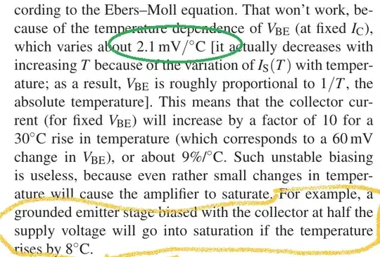
So, assuming about \$-2.1\:\text{mV}\$ change in \$V_{_\text{BE}}\$ per Kelvin rise (see citation below), one would expect to see a \$-16.8\:\text{mV}\$ change for an \$8^\circ\text{C}\$ rise. I believe that AofE also uses \$V_T=25\:\text{mV}\$ (see citation below), so this says I should expect to see \$ \frac{I_{C_2}}{I_{C_1}}\approx 1.96\$.

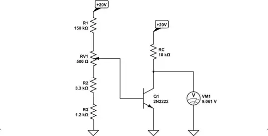
As the starting assumption says \$I_{_\text{C}}=1\:\text{mA}\$, you should then find the new \$I_{_\text{C}}\approx 1.96\:\text{mA}\$. That will produce a drop across the \$10\:\text{k}\Omega\$ collector resistor of \$19.6\:\text{V}\$. That will cause \$V_{_\text{CE}}=400\:\text{mV}\$. And that is in saturation.

This is the direct use of Ebers-Moll by the authors used to make their statement.

derivations

Before I get to the derivations, AofE 3rd edition has this chart:

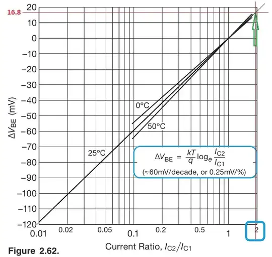
I've put a horizontal red line at about \$16.8\:\text{mV}\$ and extended the \$25^\circ\text{C}\$ line a tiny bit. There's a green arrow pointing to where these intersect. I dropped another vertical red line from there. You can see that it is very close to \$2\$. So you should expect about a doubling of current (or halving) based on this number of millivolts difference. (I said \$\frac{I_{C_2}}{I_{C_1}}\approx 1.96\$. Close enough.)

I've also circled in blue the same equation I used at the outset. So I think this is what the authors of AofE expected their readers to both work out and to apply.

But let's derive it.

First, simplify Ebers-Moll slightly: \$I_{_\text{C}}=I_{_\text{SAT}}\cdot\left(\exp\left(\frac{V_{_\text{BE}}}{V_T}\right)-1\right)\approx I_{_\text{SAT}}\cdot\exp\left(\frac{V_{_\text{BE}}}{V_T}\right)\$, as the -1 term is negligible. Then solve: \$V_{_\text{BE}}=V_T\cdot\ln\left(\frac{I_{_\text{C}}}{I_{_\text{SAT}}}\right)\$. If you have two different collector currents then:

$$\begin{align*}\Delta V_{_\text{BE}}&=V_{_{\text{BE}_2}}-V_{_{\text{BE}_1}}\\\\&=V_T\cdot\left(\ln\left(\frac{I_{_{\text{C}_2}}}{I_{_\text{SAT}}}\right)-\ln\left(\frac{I_{_{\text{C}_1}}}{I_{_\text{SAT}}}\right)\right)\\\\&=V_T\cdot\left(\ln\left(I_{_{\text{C}_2}}\right)-\ln\left(I_{_{\text{SAT}}}\right)-\ln\left(I_{_{\text{C}_1}}\right)+\ln\left(I_{_{\text{SAT}}}\right)\right)\\\\&=V_T\cdot\left(\ln\left(I_{_{\text{C}_2}}\right)-\ln\left(I_{_{\text{C}_1}}\right)\right)\\\\&=V_T\cdot\ln\left(\frac{I_{_{\text{C}_2}}}{I_{_{\text{C}_1}}}\right)\end{align*}$$

Given \$V_T=\frac{k\,T}{q}\$, there's no difference. Same thinking, same process, same end result.

All of the above, though, starts and ends with the idea that \$I_{_\text{SAT}}\$ is the same. However, it's not. In fact, that's what is changing the most when the temperature changes. (Not \$V_T\$ which only changes about 0.3% per Kelvin at room temp.)

So, if you want to get nit-picky, you could fairly complain that all of the above isn't correctly derived for the situation where temperature is changing since it assumes it isn't changing.

So that's a different question, really. Let's ask it:

$$\begin{align*} \Delta V_{_\text{BE}}&=V_{_{\text{BE}_2}}-V_{_{\text{BE}_1}} \\\\ &=V_{T_2}\cdot\ln\left(\frac{I_{_{\text{C}_2}}}{I_{_{\text{SAT}_2}}}\right) - V_{T_1}\cdot\ln\left(\frac{I_{_{\text{C}_1}}}{I_{_{\text{SAT}_1}}}\right) \end{align*}$$

Now, we can start by saying \$V_{T_1}=25\:\text{mV}\$ because that's where the authors start. We can also work out that \$V_{T_2}=25.689386661\:\text{mV}\$, because that's what happens when you add \$8^\circ\text{C}\$. We've also been given that \$\Delta V_{_\text{BE}}=-16.8\:\text{mV}\$.

So not all is buried in unknowns.

Also, we can ask "What if we assume \$I_{_{\text{C}_1}}=I_{_{\text{C}_2}}=1\:\text{mA}\$? Also assume some value for \$I_{_{\text{SAT}_1}}\$, say \$I_{_{\text{SAT}_1}}=1\:\text{fA}\$? Then how would \$I_{_{\text{SAT}_2}}\$ need to change in order to account for \$\Delta V_{_\text{BE}}=-16.8\:\text{mV}\$?"

We are asking about how the saturation current must change if we observe a base-emitter voltage change while holding the collector current constant.

This is actually a fair question and it's a question we can answer, quickly. We'd find that \$I_{_{\text{SAT}_2}}\approx 2.1\:\text{fA}\$.

In short, it means that \$I_{_{\text{SAT}}}\$ needs to about double. That's a lot and we still don't exactly understand why or if there is some equation that explains this change. But, using Ebers-Moll, this still suggests that we should expect to see \$I_{_\text{C}}\$ about double (since the Ebers-Moll saturation current multiplier just doubled due to some temperature change.)

So we can get to a similar place through different thinking.

Hopefully, this helps you realize that the AofE authors aren't just pulling stuff out of thin air.

It should also let you notice that you can just use the constant temperature Ebers-Moll slope to get a bead on what to expect, even if the assumption of constant temperature is wrong. This is because the slope is still about the same for small changes in temperature.

But you can turn things around and assume the authors are right about the change in the base-emitter voltage for that small temperature change and work backwards into what that must mean for the y-axis intercept (saturation current) and get to about the same place that way.

Just in case it still bothers you that we don't yet have a quantitative equation for temperature changes in the saturation current, here's an approximate equation from the literature:

$$I_{\text{SAT}\left(T\right)}=I_{\text{SAT}\left(T_\text{nom}\right)}\cdot\left[\left(\frac{T}{T_\text{nom}}\right)^{3}\cdot e^{^{\frac{E_g}{k}\cdot\left(\frac{1}{T_\text{nom}}-\frac{1}{T}\right)}}\right]$$

(The power of 3 is actually another model parameter as it's not always exactly 3 for all devices.)

If you apply that equation, you'll find that by itself the saturation current rises by more than a factor of 2. Perhaps almost twice that much. But this is countered by the increase in \$V_T\$. To make this point, note that \$\frac{\left(25\:\text{mV}+8^\circ\text{C}\,\cdot\, 86.173\:\frac{\mu\text{V}}{^\circ\text{C}}\right)\,\cdot\,\ln\left(\frac{1\:\text{mA}}{4\:\text{fA}}\right)-25\:\text{mV}\,\cdot\,\ln\left(\frac{1\:\text{mA}}{1\:\text{fA}}\right)}{8^\circ\text{C}}\approx -2.1\:\frac{\text{mV}}{^\circ\text{C}}\$.

(Note the use of a factor of four increase.)

And that pulls in all the unknowns together, rather than assuming one or another thing is constant. But I think you can see why it's just not done that way in engineering. Too much detail that isn't needed. Simplifying ideas combine these physical factors into a conflated mush, true, but they are also sufficient for practical use.

You will find, elsewhere in various engineering literatures, that diode leakage about doubles every \$8^\circ\text{C}\$ or \$10^\circ\text{C}\$. In broad strokes this is where that comes from. We saw just such a doubling. Here, it is forward biased. In leakage, reverse biased. But underlying Boltzmann thermodynamic statistical ideas remain.

supporting notes from AofE, 3rd edition

and,

Answer 2

Here is a simulation (made with microcap v12)

For equations, see link.

Current Is thermal dependance ...

NB: temperature behavior of "Is" ...

Appropriate values for XTI and EG depend on the type of transistor and the semiconductor material used. In practice, the values of XTI, EG, and XTB need tuning to model the exact behavior of a particular transistor.

Changing only temperature in DC Analysis ...
If you change the "beta", it does not change the behavior.
So, + 8 °C ... does "double" (quasi...) the Ic current.

Answer 3

First hint: apply Ebers-Moll to the system.

You're only given Vc, and that Vbe is fixed.

What must Vbe be, then? You won't have an exact value of course, but as a function of everything else.

Second hint: what is the tempco of Is? Vbe?

Third hint: what does "saturation" mean in terms of Ic, here?

Final hint: given that Vbe is a function of all these parameters, how much temperature change gives saturation?

Answer 4

how is this circuit biased to 0.5Vcc

From TAoE you: base-voltage-biased

The circuit is biased by attaching the base to a voltage source. In a practical circuit, the impedance of the source doesn't need to be very low, so an adjustable source with a couple kΩ of source impedance will do just fine.

^{simulate this circuit – Schematic created using CircuitLab}

Circuit is shown at room temperature with RV1 set to mid-range. It should have enough adjustment range get VC=10V with any 2N2222 at room temperature.

What's the purpose of putting 1.2k+3.3k?

Anyone who'd try to assemble this will have 1k2 and 3k3 resistors, but not 4k53 from the E96 series.

Verify that a 8°C rise in ambient temperature will cause a base-voltage-biased grounded emitter stage to saturate [that] was initially biased for Vc = 0.5Vcc

Vc=0.5Vcc means that there's about 1mA of collector current.

For a constant collector current, Vbe changes -2mV/°K. Conversely, with a constant Vbe, collector current increases with temperature. Raising the temperature by 8°K is has the same effect on collector current as raising Vbe by 16mV.

equations [...] seemingly pop up out nowhere with no explanations

What matters is that the collector current scales with \$e^{V_{BE}/V_t}\$.

At initial temperature, with some constant of proportionality \$a\$, we have approximately

$$ 1{\rm\,mA} = a \cdot e^{V_{BE}/V_t};$$

but 8°K above that we have approximately

$$\begin{aligned} I_C' &= a \cdot e^{(V_{BE}+16{\rm\,mV})/V_t} \\ &= a \cdot e^{V_{BE}/V_t + 16{\rm\,mV}/V_t} \\ &= a \cdot e^{V_{BE}/V_t} \cdot e^{16{\rm\,mV}/V_t}. \end{aligned}$$

Let's see what the ratio of collector currents in these two conditions would be:

$$ \frac{I_C'}{1{\rm\,mA}} = \frac { a \cdot e^{V_{BE}/V_t} \cdot e^{16{\rm\,mV}/V_t} } { a \cdot e^{V_{BE}/V_t} } = e^{16{\rm\,mV}/V_t} \approx e^{16{\rm\,mV}/26{\rm\,mV}} \approx 1.9. $$

So, raising the temperature by 8°C will almost double the collector current from 1mA to 1.9mA. With 1.9mA flowing through RC, the voltage drop is 19V, \$V_{CE}\$ is 1V or less, and the transistor is about to saturate. Adding the \$-1\$ term we omitted back into the Ebers-Moll formula, we get that the transistor is indeed saturated.

Answer 5

The saturation current is defined in the transistor's datasheet as Ic, with graphs showing VBE, temperature, and current.