Looking for the idea
I first thought seriously about this famous circuit solution of a constant current source three years ago when I laid out my insights in one of my questions and answers.
Now, looking again at this circuit configuration with two transistors facing each other, I struggled to find some even simpler and more logical explanation of this interlocking connection. Thus I came to the conclusion that first I need to unfold this "ball" of links and elements to distinguish some familiar functional blocks and then connect them in cascade one after the other as we usually draw schematics.
Showing the circuit evolution
Drawn in such a compact form, the circuit diagram takes up little space... but the idea remains hidden. So I realized that the best way to explain it was to show the circuit evolution step by step through CircuitLab experiments.
I have used an ammeter as a current load, changing its internal resistance manually (in the parameters window) or through the DC Sweep Simulation. Initially, its resistance is zero, hence the designation RL=0.
For convenience, in these conceptual circuits, I have tried to use "decimal" (multiples of 10) values of electrical quantities whenever possible.
Resistor current source
In principle, setting a constant current is done by connecting a resistance element in series with the load. In the simplest case, this is an ordinary constant (ohmic) resistor R. As you can see, when the load resistance is zero, the current exactly follows Ohm's law - I = Vcc/R = 10 [V]/10 [kΩ] = 1 [mA].

simulate this circuit – Schematic created using CircuitLab
But when the load resistance starts to vary (0 ÷ 10 kΩ), we see that the current does not remain constant. The greater the resistance R, the more constant the current will be, but this also requires a higher supply voltage. The problem is that the resistor is "static" (with constant resistance).
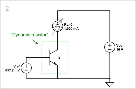
Transistor current source
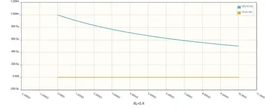
We can solve this problem with a clever trick - changing the resistance R in the opposite direction to RL so that their sum remains constant. As a result, the current will stay constant, I = Vcc/(R + RL) = const. The role of such a dynamic resistor can be played by a transistor. Its "resistance" (Vce/Ic) complements the load resistance RL so that their sum is approximately equal to 10 kΩ.
simulate this circuit
As a result, its IV curve is close to the horizontal curve of a good current source.
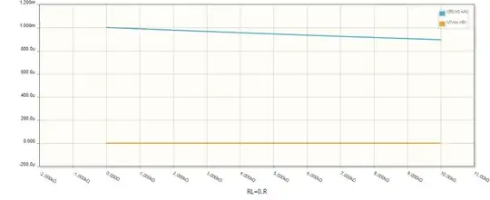
Note that ultimately the transistor is controlled by the (differential) base-emitter voltage which can be a difference of two (single-ended) voltages (Vbe = Vb - Ve). So if we raise both voltages by 1 V...
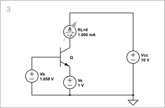
simulate this circuit
... nothing will change.
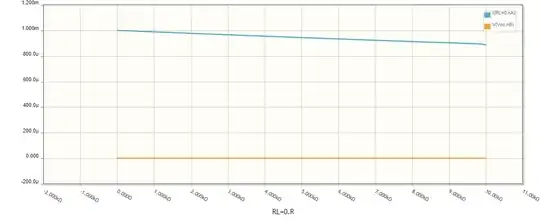
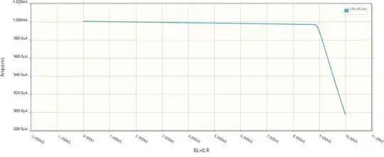
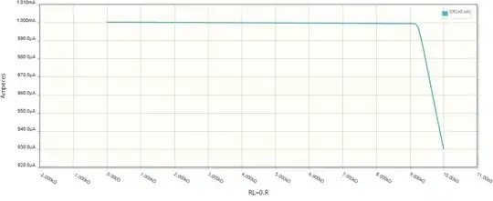
Negative-feedback current source
So far, we have exploited the transistor's property to behave as a current-stabilizing nonlinear element at a constant base-emitter voltage. It did this by changing its "resistance". But cannot we simultaneously make it change its input voltage Vbe (by changing Ve)?
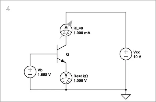
They thought of doing it a century ago and called it emitter degeneration. For this purpose, it is enough to replace the constant voltage source Ve with a "proportional source" with voltage Ve = I.Re, i.e. resistor Re (a voltmeter with 1 kΩ internal resistance). Now when RL increases, the current will try to decrease. Ve will decrease; that will increase Vbe and the current will increase (restore its previous magnitude).
simulate this circuit
The IV curve is apparantly horizontal. At RL = 9 kΩ, the transistor exhausts its supply of "resistance" (saturates), and the current decreases.
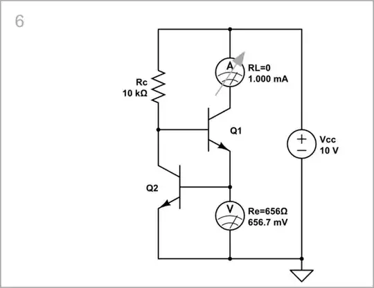
2-transistor current source
Finally we arrived at our circuit idea. Above, the transistor Q1 was "self-controlling" by changing its emitter voltage. Now we give it a chance to control its base voltage at the same time. For this purpose, we amplify Ve by another transistor Q2 and apply it to the Q1 base. Something interesting happens here - Q1 controls both Vе (direct) and Vb (amplified) at the same time. For example, if Ve tries to decrease, Vb will increase many times over and overall the input voltage Vbe will increase.

simulate this circuit
As a result of the added amplification, the IV curve becomes absolutely horizontal.
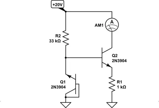
Conventional circuit diagram
Well, let's finally flip Q1 against Q2 to get the conventional compact schematic.
simulate this circuit
Voltage source
In the circuit above with a current-type negative feedback, we had to invert Ve before applying it to the base of the transistor because the stage is not-inverting. For comparison, in a transistor diode circuit there is no need for such inverting because the amplifier stage itself is inverting.
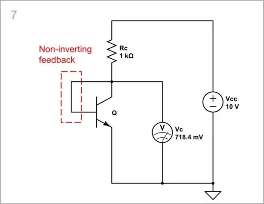
simulate this circuit
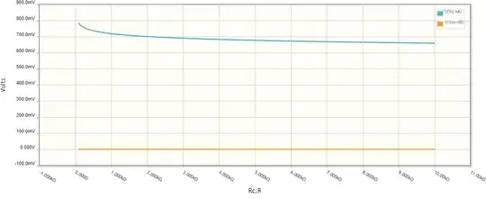
As you can see, the current-stabilizing transistor is made to act as a voltage stabilizer with an almost vertical IV curve (here it is horizontal since the voltage is plotted along the ordinate).


