One thing you should be able to see right away is that the resistor going directly from A to B may be removed before analysis, if you do these things by hand. It's directly across the terminals, so it will be in parallel with whatever you work out after first removing it. So I'm just tossing that out there in case it helps in some later practical cases.
KCL doesn't care, as it's just another graph edge. So I'll keep it for those purposes.
Here's your graph with the resistor you could remove (and later apply) circled in blue. The graph is otherwise labeled for KCL purposes below:
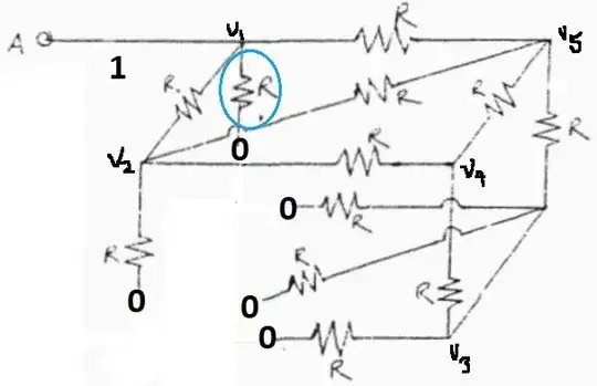
Node B has been grounded and I will inject a current of \$1\:\text{A}\$ into node A (also called \$v_1\$ above.) That will cause the voltage at \$v_1\$ to directly reflect the resistance magnitude.
I used SymPy/Python/Sagemath (all free to download and use) here.
e1 = Eq( 3*v1/R, v2/R + v5/R + 1 )               # nodal for v1 with 1 A injected
e2 = Eq( 4*v2/R, v1/R + v4/R + v5/R )            # nodal for v2
e3 = Eq( 5*v3/R, v4/R + v5/R )                   # nodal for v3
e4 = Eq( 3*v4/R, v2/R + v3/R + v5/R )            # nodal for v4
e5 = Eq( 4*v5/R, v1/R + v2/R + v3/R + v4/R )     # nodal for v5
solve( [ e1, e2, e3, e4, e5 ], [ v1, v2, v3, v4, v5 ] )[v1]
139*R/280
That's it. Feel free to ask for clarifications.
I discuss a related application of graph theory here. (KCL uses directed graph theory.) You can use graph theory to provide you directly with the meshes, if you wanted to apply mesh analysis, instead. I discuss that option there in the link (look for discussion of null spaces.)
Here's a Spice run using \$R=1\:\Omega\$:
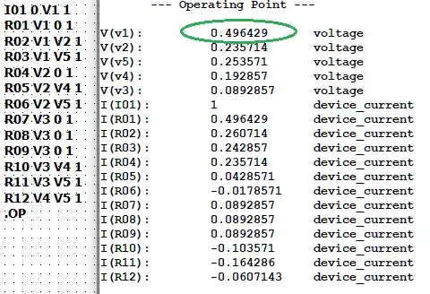
The green circled value shows the ratio and is consistent with \$\frac{139}{280}R\approx 0.496428571\,R\$ when \$R=1\:\Omega\$.


directed graph theory. – periblepsis Dec 27 '23 at 09:27