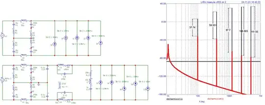
Holey moley, is that thing completely naked and unfiltered?!
The CM plot shows considerable content in this mode, with several peaks higher than in DM. You'll want to add a current source between one or both lines (use an ideal transformer to couple a single source to both lines, or use two equal sources) and GND to model this.
Note that the CM impedance is probably very high (presumably, the mains side is isolated, i.e. dominated by stray capacitance of the transformer and layout), which means the added 75µH in CM has little effect (and CX has none, by definition). Or for that matter, modeling noise as an ideal current source, the 75µH has actually zero effect, but in practice there will be some unavoidable Zcm such as stray capacitance.
It is for this reason, there is usually a Y capacitor, from primary side, to output, or to GND (in which case there must also be one from output to GND), which shunts the noise current, and reduces its source impedance, so the CMC (common mode choke) has something to work against.
Then, much larger inductance is used (~mH), to get reasonable attenuation at these relatively high impedances (fractional to low kΩ). The DM inductance tends to be smaller than shown, conveniently supplied by leakage inductance in the CMC; though if it's not enough, larger CX's or additional DM inductance (a single choke in series with either line, doesn't have to be symmetrical) may be required.
As for representation of noise sources, picking individual tones is not very convenient:
- You have to run Transient Analysis, followed by Fourier, to see the tones
- It's much harder to represent broadened or spread-spectrum sources (peak width, forest-of-peaks)
- If the tones shift due to conditions not included in the test, your simulation is invalid, and significant effort is required to correct it (i.e. re-tune all the peaks)
- It's a huge pain in general, when all you really need to input is attenuation at frequency.
And you get the last, for free (not that computation isn't almost free these days anyway, but at least in the background it is an orders-of-magnitude difference), by doing an AC steady state analysis.
Whatever filter you simulate, anyway, will only ever be poles and zeroes -- an RLC approximation of the real thing, easily constructed and solved, which since the real thing is unlikely to exhibit much transmission line / wave effect at conducted frequencies, such an approximation converges quickly.[1]
And, at low frequencies where emissions are generally strongest, simpler equivalents will suffice, thus we expect a real filter to have a dominant-pole response, with few zeroes, and we can design a filter in the usual way: pick Fc, order, input and output Z, filter prototype; look up in table, and there it is.
[1] That is, the curve fitness improves rapidly as the number of elements representing it increases. Here's a worked example: T6161-X504 (links to my site). You can see how well the curve fits mid-band, using a mere handful of components, but begins to diverge at the edges.
At higher frequencies, the lumped-element model falls apart as more and more component strays take over (the impedance curve gets more intricate, harder to model; and more dependent on component tolerances, e.g. the exact position of some stray turn of wire), and pretty soon, conducted gives way to radiated (30MHz boundary) where we care even less about the exact circuitry in play, rather that the module(s) or overall system are exhibiting these emissions and it is your challenge / responsibility to find where and how they're generated, and to motivate your changes based on whatever equivalent circuits you might construct of the local environment, whether it's noise due to risetime and ringing of switches themselves, attenuation of any points inbetween, tighter (RFI) filtering at the wires/connectors, or shielding over the board, in part or whole.
In any case, AC steady state just needs one source (say a DM current source representing converter input ripple, or a voltage source + capacitor representing the CM isolation boundary; but not both simultaneously, as they will superimpose), and you read out the gain from an approximately equivalent source to LISN at all frequencies, not just the peaks measured.
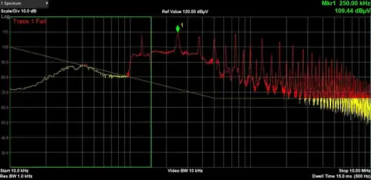 The CM noise spectrum is measured as follows:
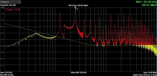 It is evident that I need large attenuation for both CM and DM.
The approach I had in mind to this problem is to create a simulation that emulates the measured noise spikes at the given frequencies (for DM and CM separately). Then add a filter that removes that type of noise and lastly reanalyze the combined DM/CM filter for DM/CM attenuation. However, when I build the simulated filter, there seems to be a rather big difference between simulation and realworld performance of the filter.
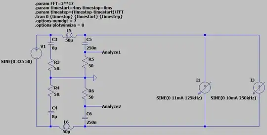 The simulation gives the following output:
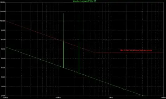 This output follows the measurement pretty close (the values of the current loads were chosen empirically to match the amplitude of the measurements). The plot is created by performing an FFT on a transient analysis and scaling the result by 1 million to convert to dBµV in stead of dbV (inspired by this video: EMC Simulation).
For reference, my FFT setting are as follows:
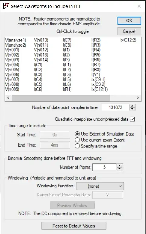
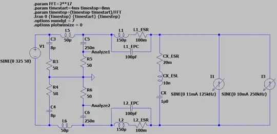 The simulation result:
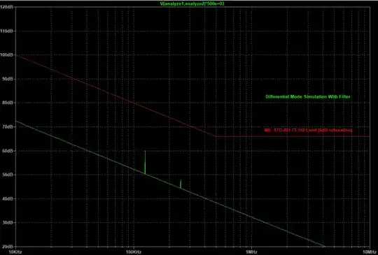 The attenuation seems to be very good with this simple filter, however the measurements that I have performed afterwards do not show a good correspondence with the simulation (the filter attenuates 20dB less than the simulation).
I would really appreciate any guidance on how to make the simulation more realistic or if anyone could point out any mistakes I have made or anything I may have missed.