While you can, technically, set up things in mesh analysis (KVL) to use composite current equations, including definitions for \$i_2\$ and \$i_3\$ for example as part of your analysis process, it's not usually done that way. Instead, those are usually developed as a result at the end of the process. So let me explain, using your own diagram:
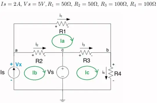
Usually, mesh is performed using the circular current loops I'm showing above in green. (I've chosen clockwise for all three loop currents.) I've labeled my mesh currents completely differently from your labels, so I can talk about your currents and mine without confusion. (I also was forced to label the voltage across \$I_s\$ as \$V_x\$, since you already have a \$V_s\$ on the schematic.)
Now, when you write that \$I_s=i_1+i_2\$ you are writing a nodal equation (KCL) and not a mesh equation (KVL.) You are right, so far as it goes. But this really isn't going to be much help, right now, if you are trying to perform a strictly mesh analysis.
For mesh purposes in the case I show above, you could write \$I_s=I_b\$ since they must be the same. (It's also true that \$i_4=I_c\$ and that \$i_1=I_a\$.)
Anyway, let's do the mesh analysis. I will start each equation from the lower-left corner and work clockwise around the loop:
$$\begin{align*}
0\:\text{V}-R_1\cdot I_a -R_3\cdot\left(I_a-I_c\right)-R_2\cdot\left(I_a-I_b\right)&=0\:\text{V}
\\\\
0\:\text{V}+V_x-R_2\cdot\left(I_b-I_a\right)-V_s&=0\:\text{V}
\\\\
0\:\text{V}+V_s -R_3\cdot\left(I_c-I_a\right)-R_4\cdot I_c&=0\:\text{V}
\end{align*}$$
Now, that looks initially like three equations with four unknowns. But, in fact, you already know that \$I_b=I_s\$. So it's really just three equations with three unknowns.
Let's use freely available SymPy:
# the imports I have from my 'init.sage' file:
from sympy import *
from sympy.solvers import solve
from sympy import radsimp, signsimp
from sympy.simplify.radsimp import collect_sqrt
now follow along:
ia,ib,ic,vs,vx,r1,r2,r3,r4 = symbols( 'ia,ib,ic,vs,vx,r1,r2,r3,r4', real=True )
e1 = Eq( 0 - r1ia - r3(ia-ic) - r2(ia-ib), 0 )
e2 = Eq( 0 + vx - r2(ib-ia) - vs, 0 )
e3 = Eq( 0 + vs - r3(ic-ia) - r4ic, 0 )
ans = solve( [e1, e2, e3], [vx, ia, ic] )
specific = { r1:50, r2:50, r3:100, r4:100, vs:5, ib:2 }
for item in ans: item, ans[item].subs(specific), ans[item].subs(specific).n()
(vx, 425/6, 70.8333333333333)
(ia, 41/60, 0.683333333333333)
(ic, 11/30, 0.366666666666667)
From the above, you can now work out the resistor currents (which are composed from the now-analyzed mesh currents) as \$i_1=I_a\approx 683.3\:\text{mA}\$, \$i_2=I_b-I_a\approx 1.3167\:\text{A}\$, \$i_3=I_c-I_a\approx -316.7\:\text{mA}\$, and \$i_4=I_c\approx 366.7\:\text{mA}\$.
In short, you work out the net device currents from the mesh currents after you figure those out, first.
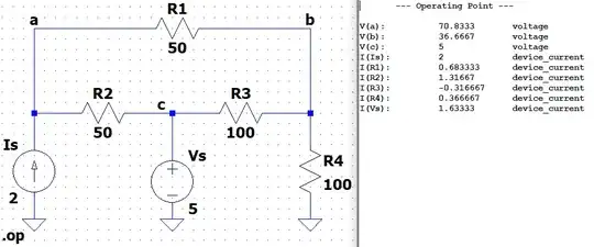
Here's a Spice .OP run of the above so as to "trust, but verify":