Overview
This is an interesting circuit.
Partly, because it breaks down into parts we all recognize: an RC filter, a follower, and the 1st stage which is also a fairly familiar differential amplifier.
I really enjoyed looking over the analysis already here, as well as yours.
You wrote \$V_1 = \frac{R_2}{R_1+R_2} U_o\$ and I immediately mentally noted that since \$V_1=V_2\$ that it must also be equal to \$V_2=\frac{V_s\,\cdot\,R_1+V_3\,\cdot\,R_2}{R_1+R_2}\$. Equating them suggests that \$R_2\cdot V_o=V_s\,\cdot\,R_1+V_3\,\cdot\,R_2\$.
But then I backed off to just look at it, more.
Perhaps a way to see the circuit is to start at the capacitor. The follower buffers the capacitor voltage and feeds it immediately into the differential as the positive input. Given the resistors shown, a proportion of the input is subtracted from the capacitor voltage to set the output at \$V_3\$. The \$R\$ sets the output impedance as resistive (real axis) and the capacitor itself is orthogonal to it (imaginary axis.) This is important as it means the output will be chasing the input.
If a DC input is provided, then the difference will always have the same sign and the capacitor will simply force the opamps to ramp towards hitting their rails. But if AC is provided, then the chasing process continues ever around the circle.
Using Solver
In any case, I decided to just sit down and let the KCL stuff flow out, leaving the gnarly algebra to SymPy:
eq1 = Eq( v1/r1 + v1/r2, vo/r1 )                 # KCL node 1
eq2 = Eq( v2/r2 + v2/r1, vi/r2 + v3/r1 )         # KCL node 2
eq3 = Eq( v3/r1 + v3/r, io1 + v2/r1 + v4/r )     # KCL node 3
eq4 = Eq( v4/r + v4/(1/s/c), v3/r )              # KCL node 4
eq5 = Eq( vo/r1, io2 + v1/r1 )                   # KCL output node
eq6 = Eq( v1, v2 )                               # 1st opamp requirement
eq7 = Eq( v4, vo )                               # 2nd opamp requirement
simplify( solve( [ eq1, eq2, eq3, eq4, eq5, eq6, eq7 ], [ v1, v2, v3, v4, vo, io1, io2 ] )[vo] / vi )
-r1/(c*r*r2*s)
So, this tells me that the transfer function is \$\frac{-R_1}{R\,\cdot \,R_2\,\cdot\,C}\cdot\frac1s\$. So it seems, anyway.
In the time domain, I believe this would translate into \$\frac{-R_1}{R\,\cdot \,R_2\,\cdot\,C}\int_{_0}^{^t}V_t\:\text{d}t\$. And if we limit ourselves to a sinusoidal \$V_t=V_{_0}\cdot\cos\left(\omega \cdot t\right)\$ then it works out to \$\frac{-R_1}{R\,\cdot \,R_2\,\cdot\,C}\cdot V_{_0}\cdot\frac1{\omega}\cdot\sin\left(\omega \cdot t\right)\$.
In short, I should expect to see a voltage gain that is inversely proportional to frequency. And I mean inversely. There's no near-DC flat-top here. As you get near to DC the gain grows without bound.
I should also tend to see the opamps hitting their rails with very low frequencies and diminishing towards 0 at very high frequencies. The difference between this and a standard low-pass RC is that in this case applying a non-zero DC voltage results in a ramp towards one of the rails where it will ultimately just sit. In contrast, a low-pass RC would just present a copy of the applied DC voltage. (Except for 0, that doesn't happen here. It just integrates.)
Apply Theory
Okay. That is what I did before attempting to see what LTspice would say to me. So I set down to specify some values to use and then proceeded to make some predictions from them.
(This is what I do in my engineering logbook -- always develop the theory first, make some explicit predictions from that theory, and then go test it and write down those results, as well. That way I can tell where I fail and where I succeed and this helps me learn. It also gives me a way to look back on where I have made mistakes.)
I'll use \$R_1=10\:\text{k}\$, \$R_2=30\:\text{k}\$, \$R=10\:\text{k}\$, \$C=15.9\:\text{nF}\$ and \$V_{_0}=1\:\text{V}\$.
I am predicting a voltage gain of \$\frac{2096.43606}{\omega}\$ for this configuration.
Test Theory
I'll now wire up a schematic in LTspice. I tend to use their LT1800 because it's just a generally good (and too expensive for me) device with rail-to-rail support and a behavioral model that seems to run well for me. So I'll use that.
Let's try a frequency of \$300\:\text{Hz}\$ first. In this case, I'd predict a voltage gain of \$\approx 1.1\$:
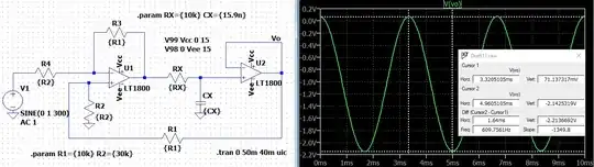
This shows that the peak-to-peak output is \$\approx 2.2\:\text{V}\$. With an input peak-to-peak of \$2\:\text{V}\$ and a voltage gain of \$\approx 1.1\$ that seems amazingly close.
Let's try a frequency of \$600\:\text{Hz}\$ next. In this case, I'd predict half the earlier voltage gain, or \$\approx 0.55\$:
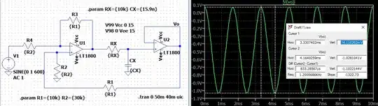
And here we see the peak-to-peak output is \$\approx 1.1\:\text{V}\$. As expected.
One final try at a frequency of \$1\:\text{kHz}\$. In this case, I'd predict a voltage gain of \$\approx \frac13\$:
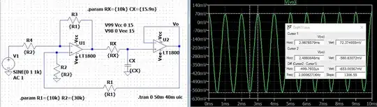
And there it is; the peak-to-peak output is \$\approx 650\:\text{mV}\$. As expected.
My logbook is complete on this, I guess.
Added
The following is how I mentally visualized what I just wrote, earlier, in the Overview. I tried to use words there, but here's the mental picture that was in my mind while I was writing it:
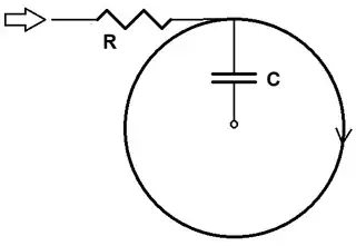
For larger values of \$\omega\$ the reactance of the capacitor has a smaller value and therefore the radius of the above circle is similarly tighter/smaller, and the magnitide is therefore smaller. The differentially-arranged opamp is pushing on \$R\$, which causes the rotation. But no matter how hard it tries, \$R\$ is always positioned to be tangent to the \$C\$-axis, so all the pushing does is to just continue the rotation.
I admit that the \$R\$ and \$C\$ on your schematic was nicely arranged for me to see this circle superimposed on it when I was first reading it. I actually super-imposed the circle, mentally, then. ;)
The rest of the circuit is all resistive and fast. So it can be mentally lumped in mind as instantaneous. (Ignore any delays.)
Also, the schematic you have really will need (if you build one) a small capacitance (maybe \$22\:\text{pF}\$?) across the feedback resistor of the differentially-arranged 1st stage opamp. It's common practice, though. Just FYI.


