In lieu of a schematic as yet, I will take the most obvious interpretation I suspect given the comments:
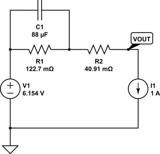
simulate this circuit – Schematic created using CircuitLab
A Thevenin voltage source, where the impedance is, not just a series resistance, but an (R || C) + R, with the values shown derived from the plots given.
This was determined by the following procedure:
(1) Extract Current Waveform
In lieu of a data series, a curve was fitted. The nearly flat initial segment suggests a time delay of about 3µs, and the fairly smooth curve suggests an RLC equivalent response. An exponential polynominal was therefore used:
$$ i(t) = \begin{cases} i_0 & t < 0 \\ i_0 + A \left( e^{\frac{-t}{\tau_a}} - 1 \right) + B t e^{\frac{-t}{\tau_b}} + C t^2 e^{\frac{-t}{\tau_c}} & t \ge 0 \end{cases} $$
Where,
$$
\begin{array} \\
i_0 &= 3.852 \, A\\
i_s & = -0.275 \, A\\
A &= 0.275\, A\\
\tau_a &= 1 \, \mu s \\
B &= 0.15\, A\\
\tau_b &= 1 \, \mu s \\
C & = -0.0181 \, A\\
\tau_c & = 2.82 \, \mu s \\
\end{array}$$
Finally, 2.7µs was subtracted off to get the correct time offset.
This is assumed to be I1 in the above schematic (not a fixed current as shown, but a dependent signal current as above).
(2) Fit Voltage Waveform
The circuit elements were solved by fitting to the voltage curve. Whereas the above method uses an analytic form suggestive of an RLC network transient response, this function is assumed to have a filtering action upon that waveform. Which requires calculating the convolution of impulse responses, in the time domain: not something I'm going to do in Excel, and not trivial in the analytic form. (At least, I don't feel like writing it out to solve it based on circuit values.) Therefore, an incremental method was chosen.
First, a parallel RC was suspected. This was found to fit a bit poorly during the rising edge, with error seemingly proportional to current. Therefore, series resistance was added, and this seems to reduce error to acceptable levels. Remaining error appears fairly random, or perhaps a higher frequency interfering signal (ca. 50 kHz).
The method chosen was calculation by forward difference, i.e., evaluating the differential system as a fixed-timestep difference equation, also known as Newton integration. First, a finer timestep was chosen, to help avoid numerical error. Then the recurrence relation was entered, solving for the state variable, C1's voltage:
$$ v_c[n] = v_c[n-1] + \left( i[n] - \frac{v[n-1]}{R} \right) \frac{t_s}{C} $$
Where \$v_c[n]\$ corresponds to \$v_c(n t_s )\$, the voltage on C1, and \$t_s\$ is in µs, R in Ω, and C in µF. Finally, these voltages (the capacitor voltage, and the voltage drop on R2 which is simply proportional to current, not shown here) were subtracted from the source, to give the output plot. These values were found suitable:
$$
\begin{array} \\
t_s & = 0.05 \, \mu s \\
V_1 & = 6.154 \, V \\
R_1 & = 0.1223 \, \Omega \\
R_2 & = 0.04091 \, \Omega \\
C_1 & = 88 \, \mu F \\
\end{array}$$
The result is shown below:
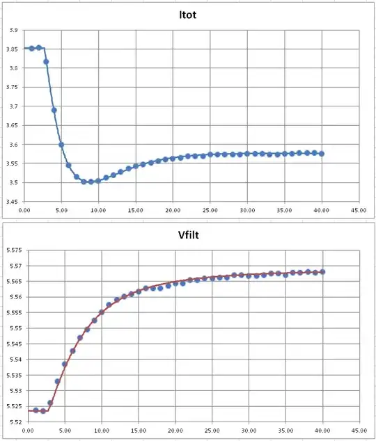
Entering these formulas into Excel and using SOLVER to reduce the (peak or RMS) differences between measured values and fitting curves, is one method to automate this process. Presumably, the circuit will not change with bias, so a range of values can be calculated fairly straightforwardly in this way. (Further fitting could be applied to solve for R and C's as a function of V and I.)
Copy of worksheet can be found here: https://docs.google.com/spreadsheets/d/1UlApQS7rQfDtFgXMhounzrgPsHOYUSxV/edit?usp=sharing&ouid=114876650507578990049&rtpof=true&sd=true


