Why the output voltage of a transfer function is not equal to zero
when the exciting signal is at the frequency of the zero
Setting the denominator to 1 (because you are talking about the zero conditions rather than poles), we get: -
$$H(s) = 1+\dfrac{s}{\omega_z}$$
And, if the imaginary part of s is chosen to be \$j\omega_z\$, the transfer function is: -
$$H(s) = 1+j$$
And clearly that isn't zero but, how to find a value of s that produces a zero?
To make this happen means we have to set the TF to zero and solve for s in its general form: -
$$0 = 1+\dfrac{\alpha+j\omega}{\omega_z}$$
$$-1 = \dfrac{\alpha+j\omega}{\omega_z}$$
$$-\omega_z = \alpha+j\omega$$
$$j\omega = -\alpha - \omega_z$$
But, in the real world of signal generators, oscilloscopes and bode plots, we cannot make our signal like that; the "zero" does occur, but not along any axis we can see on a bode plot. If you plotted the pole zero diagram (this of course includes an axis for \$\sigma\$ as well as \$j\omega\$) you would see it. But, the pole zero diagram is really an abstraction from the real world and, is mathematically useful but only if you grasp it.
Fourier is along the \$j\omega\$ axis and, Laplace is the fuller story to put it simply.
For instance, an example diagram I have shows the bode plot of a 2nd order low pass filter and the pole-zero diagram combined: -
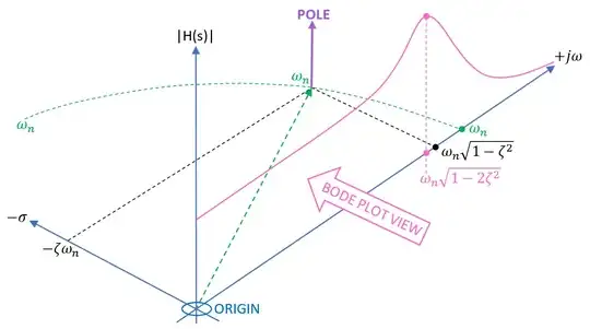
If you looked at the bode plot part (our real world of oscilloscopes and generators) you would see this: -
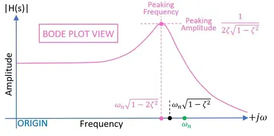
And behind the bode plot (into the page so to speak) you can see a pole. In other words, what we see in the world of oscilloscopes and signal generators is just a thin slice of a bigger mathematical picture called the pole zero diagram.

