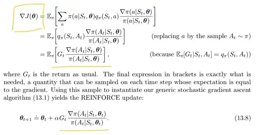
The first part of this answer is a little background that might bolster your intuition for what's going on. The second part is the more practical and direct answer to your question.
The gradient is just the generalization of the derivative to multivariable functions. The gradient of a function at a certain point is a vector that points in the direction of the steepest increase of that function.
Usually, we take a derivative/gradient of some loss function $\mathcal{L}$ because we want to minimize that loss. So we update our parameters in the direction opposite the direction of the gradient.
$$\theta_{t+1} = \theta_{t} - \alpha\nabla_{\theta_t} \mathcal{L} \tag{1}$$
In policy gradient methods, we're not trying to minimize a loss function. Actually, we're trying to maximize some measure $J$ of the performance of our agent. So now we want to update parameters in the same direction as the gradient.
$$\theta_{t+1} = \theta_{t} + \alpha\nabla_{\theta_t} J \tag{2}$$
In the episodic case, $J$ is the value of the starting state. In the continuing case, $J$ is the average reward. It just so happens that a nice theorem called the Policy Gradient Theorem applies to both cases. This theorem states that
$$\begin{align}
\nabla_{\theta_t}J(\theta_t) &\propto \sum_s \mu(s)\sum_a q_\pi (s,a) \nabla_{\theta_t} \pi (a|s,\theta_t)\\
&=\mathbb{E}_\mu \left[ \sum_a q_\pi (s,a) \nabla_{\theta_t} \pi (a|s,\theta_t)\right].
\end{align}\tag{3}
$$
The rest of the derivation is in your question, so let's skip to the end.
$$\begin{align}
\theta_{t+1} &= \theta_{t} + \alpha G_t \frac{\nabla_{\theta_t}\pi(A_t|S_t,\theta_t)}{\pi(A_t|S_t,\theta_t)}\\
&= \theta_{t} + \alpha G_t \nabla_{\theta_t} \ln \pi(A_t|S_t,\theta_t)
\end{align}\tag{4}$$
Remember, $(4)$ says exactly the same thing as $(2)$, so REINFORCE just updates parameters in the direction that will most increase $J$. (Because we sample from an expectation in the derivation, the parameter step in REINFORCE is actually an unbiased estimate of the maximizing step.)
Alright, but how do we actually get this gradient? Well, you use the chain rule of derivatives (backpropagation). Practically, though, both Tensorflow and PyTorch can take all the derivatives for you.
Tensorflow, for example, has a minimize() method in its Optimizer class that takes a loss function as an input. Given a function of the parameters of the network, it will do the calculus for you to determine which way to update the parameters in order to minimize that function. But we don't want to minimize. We want to maximize! So just include a negative sign.
In our case, the function we want to minimize is
$$-G_t\ln \pi(A_t|S_t,\theta_t).$$
This corresponds to stochastic gradient descent ($G_t$ is not a function of $\theta_t$).
You might want to do minibatch gradient descent on each episode of experience in order to get a better (lower variance) estimate of $\nabla_{\theta_t} J$. If so, you would instead minimize
$$-\sum_t G_t\ln \pi(A_t|S_t,\theta_t),$$
where $\theta_t$ would be constant for different values of $t$ within the same episode. Technically, minibatch gradient descent updates parameters in the average estimated maximizing direction, but the scaling factor $1/N$ can be absorbed into the learning rate.
