R6.1
Solved by Daniel Suh
R6.2
Problem Statement
Solve the problems 11 and 12 from Kreyszig p.491
Solution
First, for problem 11:
 from
from  where
where  We know that
  so that
We check is the function is even, odd or neither.
Since  satisfies the condition
  we know that the function is even.
Given that the function is even and that  for even functions, we exclude the
  term from the Fourier Series.
We find  :
:

Plugging in,
![{\displaystyle a_{0}={\frac {1}{2}}\int _{-1}^{1}x^{2}dx={\frac {1}{2}}\left[{\frac {1}{3}}x^{3}\right]_{-1}^{1}={\frac {1}{2}}\left[{\frac {1}{3}}+{\frac {1}{3}}\right]={\frac {1}{3}}\!}](../../9cdcec4b23b99a873211496d4c7284a7e126a84d.svg)
We find 


We can use the equivalent expression:

Now we evaluate the integral by using integration by parts. Below are the steps:
Integration by parts uses 

Then, we have:
![{\displaystyle \left[{\frac {x^{2}sin(\pi nx)}{\pi n}}\right]_{0}^{1}-{\frac {2}{\pi n}}\int _{0}^{1}xsin(\pi nx)dx\!}](../../bad33c22c5b16e79133262bd5ec55d4edda8aad9.svg)
Repeating for the second term:

Then, we have:
![{\displaystyle \left[{\frac {-xcos(\pi nx)}{\pi n}}\right]_{0}^{1}-{\frac {1}{\pi n}}\int _{0}^{1}cos(\pi nx)dx\!}](../../83b10de0d3425337dcfd8d80e144e393d55c673a.svg)
Bringing all the terms together:
![{\displaystyle 2\left[\left[{\frac {x^{2}sin(\pi nx)}{\pi n}}\right]_{0}^{1}-{\frac {2}{\pi n}}\left[{\frac {-xcos(\pi nx)}{\pi n}}\right]_{0}^{1}-{\frac {1}{\pi n}}\int _{0}^{1}cos(\pi nx)dx\right]\!}](../../a60b2f09abdff1de7c5f4edcb367187a52ca5cb2.svg)
Then,
![{\displaystyle 2\left[\left[{\frac {x^{2}sin(\pi nx)}{\pi n}}\right]_{0}^{1}-{\frac {2}{\pi n}}\left[{\frac {-xcos(\pi nx)}{\pi n}}\right]_{0}^{1}-{\frac {1}{\pi n}}\left[{\frac {sin(\pi nx)}{\pi n}}\right]_{0}^{1}\right]\!}](../../285797fa8a188f052f64069a7fb8e60d99fabecb.svg)
Evaluating at the boundaries and simplifying:
![{\displaystyle 2\left[\left[0-0\right]+{\frac {2}{\pi ^{2}n^{2}}}\left[cos(\pi n)\right]-{\frac {1}{\pi n}}\left[0-0\right]\right]\!}](../../40e36f0954f238cf8f595c4bd95b1cef757d0a54.svg)
Further,

We can simplify one step further by acknowledging that  .
.

Finally,

The Fourier series is:

Now problem 12:
 from
from  where
We know that
where
We know that  so that
We check is the function is even, odd or neither.
Since satisfies the condition we know that the function is even.
Given that the function is even and that for even functions, we exclude the term from the Fourier Series.
We find :
Plugging in,
![{\displaystyle a_{0}={\frac {1}{4}}\int _{-2}^{2}1-{\frac {x^{2}}{4}}dx={\frac {1}{4}}\left[x-{\frac {1}{12}}x^{3}\right]_{-2}^{2}={\frac {1}{4}}\left[{\frac {24-8}{12}}-{\frac {24+8}{12}}\right]={\frac {2}{3}}\!}](../../35f2149448f2c8078f965e3d71d3e3d957077c8b.svg)
We find

Now we evaluate the integral by using integration by parts. This process is similar to the one shown in the solution for problem 11 above and therefore will be performed in Wolfram Alpha.
The following command was given in Wolfram Alpha: integral (1-(x^2/4))*cos(pi*x) from -2 to 2.
Wolfram Alpha yields the following

Finally,
The Fourier series is:

Part B
Solved by Francisco Arrieta
Problem Statement
Find the Fourier series expansion for on p. 9.8 as follows:
Part 1
Develop the Fourier series expansion of 
Plot and the truncated Fourier series 
![{\displaystyle f_{n}({\bar {x}}):={\bar {a}}_{0}+\sum _{k=1}^{n}[{\bar {a}}_{k}\cos k\omega {\bar {x}}+{\bar {b}}_{k}\sin k\omega {\bar {x}}]\!}](../../b888e20b56e5edf65b6488f76ee37ceb4513bc47.svg)
for n=0,1,2,4,8. Observe the values of at the points of discontinuities, and the Gibbs phenomenon. Transform the variable so to obtain the Fourier series expansion of
Solution


Note:
If k is even 
If k=1, 5, 9... 
If k=3, 7, 11... 

Note:
 for n=1, 2...
Then Fourier series becomes a Fourier cosine series:

For n=0

For n=1

For n=5

After transforming the variable of

Part 2
Do the same as above, but using  to obtain the Fourier expansion of ; compare to the result obtained above
R6.3
Problem Statement
Page 491, #15,17. Plot the truncated Fourier series for n=2,4,8.
Solution
15.

Since  , the function is odd.
![{\displaystyle a_{0}=(1/\pi )*[-1\int _{-\pi }^{-\pi /2}(x+\pi )dx+\int _{-\pi /2}^{\pi /2}(x)dx+\int _{\pi /2}^{\pi }(\pi -x)dx]}](../../a3515ec49fdd8ef95aedb6e74ee844ba7b39b6ce.svg)
After simplification, 
.
Using Equation (5) on page 490, the exapansion becomes;

With  this becomes;
 for n is "odd".
This means when n is even, 
17.


![{\displaystyle a_{0}=1/2[\int _{-1}^{0}(1+x)dx+\int _{0}^{1}(1-x)dx]}](../../663792d020231d208ed32b73f0c4db7045053632.svg)
![{\displaystyle a_{0}=1/2[1-1/2+1-1/2]}](../../57762d639f689e1bcd7d58eeb81c3590c3473f73.svg)

![{\displaystyle a_{n}=1/1[\int _{-1}^{0}(1+x)cos(n\pi *x/1)dx+\int _{0}^{1}(1-x)cos(n\pi *x/1)dx]}](../../ecc54c05805473116b69ac5965dd79d368827f34.svg)
Simplifying results in;
![{\displaystyle a_{n}=2[1/(n^{2}\pi ^{2})_{(}-1)^{n}/(n^{2}\pi ^{2})]}](../../82a4babc3b94dfce840755f8704669ff666085ce.svg)
So,

when n is odd.
![{\displaystyle b_{n}=1/1[\int _{-1}^{0}(1+x)sin(n\pi *x/1)dx+\int _{0}^{1}(1-x)sin(n\pi *x/1)dx]}](../../9b3a3c83592e4975230374d189014a6e9669263f.svg)
Simplifying results in;


Since  for even n,
  becomes
  for even n.
R6.4
solved by Luca Imponenti
Problem Statement
Consider the L2-ODE-CC (5) p.7b-7 with the window function f(x) p.9-8 as excitation:

and the initial conditions

1. Find  such that:

with the same initial conditions as above.
Plot for  for x in
 ![{\displaystyle [0,10]\!}](../../7afee0f848455b66aae9ef3f95de42d3509f2f26.svg)
2. Use the matlab command ode45 to integrate the L2-ODE-CC, and plot the numerical solution to compare with the analytical solution.
- Level 1:

Fourier Series
One period of the window function p9.8 is described as follows

From the above intervals one can see that the period,  and therefore
Applying the Euler formulas from
and therefore
Applying the Euler formulas from  to
to  the Fourier coefficients are computed:


The integral from  to
to  can be omitted from this point on since it is always zero.


and


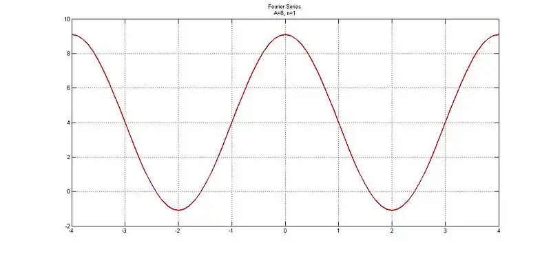
The coefficients give the Fourier series:
![{\displaystyle f(x)=a_{0}+\sum _{n=1}^{\infty }[a_{n}cos({\frac {n\pi x}{L}})+b_{n}sin({\frac {n\pi x}{L}})]\!}](../../1882b82559d4f1569411c84a2b6e3d86f161f7fe.svg)

![{\displaystyle +{\frac {A}{n\pi }}(cos({\frac {n\pi }{8}})-cos({\frac {9n\pi }{8}}))sin({\frac {n\pi x}{2}})]\!}](../../8893708df79a090f008049edab53aed382f0f66e.svg)
Homogeneous Solution
Considering the homogeneous case of our ODE:

The characteristic equation is


Therefore our homogeneous solution is of the form

Particular Solution
Considering the case with f(x) as excitation

![{\displaystyle +(cos({\frac {k\pi }{8}})-cos({\frac {9k\pi }{8}}))sin({\frac {k\pi x}{2}})]\!}](../../5cd6ccf84a4564bffcd87fc35ab5fb5eccc20fad.svg)
The solution will be of the form

Taking the derivatives


Plugging these back into the ODE:

![{\displaystyle +{\frac {\pi }{2}}\sum _{k=2}^{n}B_{k}kcos({\frac {k\pi x}{2}})]+2[A_{0}+\sum _{k=1}^{n}A_{k}cos({\frac {k\pi x}{2}})+\sum _{k=1}^{n}B_{k}sin({\frac {k\pi x}{2}})]\!}](../../fc340f38bcb387f8388802845e941835a8138559.svg)
![{\displaystyle ={\frac {A}{2}}+\sum _{k=1}^{n}{\frac {A}{k\pi }}[(sin({\frac {9k\pi }{8}})-sin({\frac {k\pi }{8}}))cos({\frac {k\pi x}{2}})+(cos({\frac {k\pi }{8}})-cos({\frac {9k\pi }{8}}))sin({\frac {k\pi x}{2}})]\!}](../../6c55a889240e8411f80b6f6e1b9954e45d32b4c8.svg)
Setting the two constants equal


This is valid for all values of n. Since the coefficients of the excitation  and
and  are zero for all even n, then the coefficients
  and
and  will also be zero, so we must only find these coefficients for odd n's.
Now carrying out the sum to
will also be zero, so we must only find these coefficients for odd n's.
Now carrying out the sum to  and comparing like terms yields the following sets of equations. Written in matrix form:

Assuming  this matrix can be solved to obtain

For the remaining coefficients to be solved all sums will be used so a more general equation may be written:

Results of these calculations are shown below:

The solution to the particular case can be written for all n (assuming A=1):

General Solution
The general solution is

where
Different coefficients  will be calculated for each n. These coefficients are easily solved for by applying the given initial conditions. Below are the calculations for n=2.

Applying the first initial condition 

Taking the derivative

Applying the second initial condition 

Solving the two equations for two unknowns yields:

So the general solution for n=2 is:

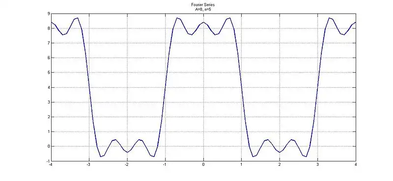
Below is a plot showing the general solutions for n=2,4,8:
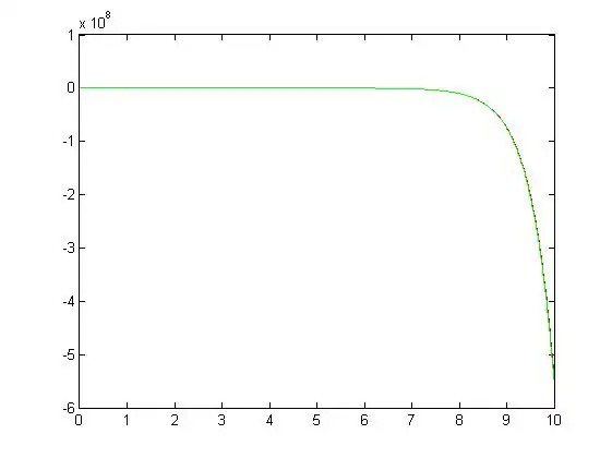

Matlab Plots
Using ode45 the following graph was generated for n=0:
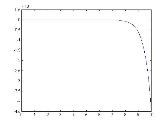
and for n=1

R6.5
Solved by: Gonzalo Perez
Part R4.2, p.7c-26
For each value of n=3,5,9, re-display the expressions for the 3 functions  , and plot these 3 functions separately over the interval
 ![{\displaystyle [0,20\pi ]\!}](../../0265ce74a1f75468b07b65508ca66e583cf31727.svg) .
.
R4.2 p.7-26: Consider the L2-ODE-CC (5) p.7b-7 with  as excitation:
 (5)p.7-7
 (1)p.9-15
and the initial conditions:
 (3b)p.3-7
Exact solution:  (2)p.9-15
Re-display the expressions for  .
.
Superpose each of the above plot with that of the exact solution.
Solution
The graphs are to be separately graphed as follows.
For n = 3, the code that will generate the graph looks like this:
For n = 6:
For n = 9:
Part R4.3, p.7c-28
Understand and run the TA's code to produce a similar plot, but over a larger interval . Do zoom-in plots about the points  and comment on the accuracy of different approximations.
R4.3 p.7-28: Consider the L2-ODE-CC (5) p.7b-7 with  as excitation:
(5)p.7-7
 (1)p.7-28
and the initial conditions:
 (2)p.7-28
Solution
For n=4 (from x = 0 to x = 10):
For n=4 (zoom-in plots around x = -0.5):
For n=4 (zoom-in plots around x = 0):
For n=4 (zoom-in plots around x = +0.5):
For n=7 (from x = 0 to x = 10):
For n=11 (from x = 0 to x = 10):
Where the black line represents n=11 and the blue line represents log(1+x).
The problem asks for n=4, 7, and 11. The TA had up to n=16, but the problem does not ask for this. Manipulating the code and graphs to only account for these n values, n=16 has been disregarded.
Combined plots for n=7 and n=11 (zoom-in plots around x = -0.5):
Combined plots for n=7 and n=11 (zoom-in plots around x = 0):
Combined plots for n=7 and n=11 (zoom-in plots around x = 0.5):
Part R4.4, p.7c-29
Understand and run the TA's code to produce a similar plot, but over a larger interval ![{\displaystyle [0.9,10]\!}](../../9c86a6f6483bf9ba445c11cb83d4e369f736f9cc.svg) , and for n=4,7. Do zoom-in plots about
, and for n=4,7. Do zoom-in plots about  and comments on the accuracy of the approximations.
R4.4 p.7-29: Extend the accuracy of the solution beyond  .
.
Solution
The general code that can be used to graph the plots of n=4,7,11 is:
With the above code, we can add the following code to graph n=4.
For n = 4 (from x = 0.9 to x = 10):
For n = 7 (from x = 0.9 to x = 10):
For n=11 (from x = 0.9 to x = 10):
Repeating the same common part of the code, let's graph the other plots around x = 1, 1.5, 2, 2.5:
For n = 4, 7, 11 at x = 1:
For n = 4, 7, 11 at x = 1.5:
For n = 4, 7, 11 at x = 2:
For n = 4, 7, 11 at x = 2.5:
For the last part, the first (and unchanged TA's code) is the following:
The second part includes the change that had to be made in order to solve this problem:


![{\displaystyle a_{0}={\frac {\omega }{2\pi }}[{\frac {sin(n\omega x)}{n\omega }}|_{-{\frac {\pi }{\omega }}}^{\frac {\pi }{\omega }}]\!}](../../948cfb833c24a8531890b3ac3410eb6e71569a99.svg)
![{\displaystyle a_{0}={\frac {\omega }{2\pi }}[{\frac {2sin(n\pi )}{n\omega }}]\!}](../../91e23e4538e88251593b0a0c69cd95afe7ce8952.svg)


![{\displaystyle a_{0}={\frac {\omega }{2\pi }}[{\frac {cos(n\omega x)}{n\omega }}|_{-{\frac {\pi }{\omega }}}^{\frac {\pi }{\omega }}]\!}](../../2eba41982a5c9a4390f37c5904e426055cbc52b4.svg)
![{\displaystyle a_{0}={\frac {\omega }{2\pi }}[{\frac {-cos{n\pi }+cos{n\pi }}{n\omega }}]\!}](../../dfa42c9d3dba92ee2ccc1ea8a835a5fe220bcfb2.svg)


