Linear algebra (Osnabrück 2024-2025)/Part II/Lecture 43
- Polynomials in several variables and their zero sets
As an application of the diagonalizability of symmetric matrices (and of principal axis transformation), we discuss how to transform simple polynomial equations in several variables of low degree to a very simple form. For this, we introduce briefly polynomials in several variables.


The degree of a monomial is the sum of the exponents, that is, .


The degree of a polynomial is the maximum of the degrees of the monomials involved (meaning those monomials that occur with a coefficient different from ). A polynomial in variables over defines a function by inserting (substituting each variable by certain values)


These are important functions in higher-dimensional analysis. The variable , interpreted in this way, is simply the -th projection, and the addition and the multiplication of polynomials corresponds to the addition and the multiplication of functions, where the values in are added or multiplied.

For a field and a set of variables , the polynomial ring
![{\displaystyle K[X_{1},\ldots ,X_{n}]}](../../3d1ac7a7496de3efbb2cd22c42398736c86a2b48.svg)
consists of all polynomials in these variables. This set is made into a commutative ring by componentwise addition and by the multiplication that extends the rule


Let be a field, and let denote a polynomial in Variables. The set
![{\displaystyle {}F\in K[X_{1},\ldots ,X_{n}]}](../../eb9907eef7712dd23f5765db372457691aa7d626.svg)

is called the vanishing set (or zero set)
of .Thus, the vanishing set of is just the fiber of the function

given by . For , this is just a finite collection of points, the zeroes of , (in case , it is ); however, for , these vanishing sets are interesting and complicated geometric objects. The study of these objects is called algebraic geometry. In case of , we talk about algebraic curves.


For arbitrary , a polynomial of degree has the form


and the corresponding vanishing set is just the solution set of the inhomogeneous linear equation

that is, it is an affine-linear space.
- Real quadrics
The polynomials of degree two and their zero-sets can be understood completely with methods from linear algebra.

A quadratic polynomial over a field is a polynomial of degree ; that is, an expression of the form


where
.
For a quadratic polynomial in one variable , with and , the zeroes can be found by completing the square. That is, we write (suppose that the characteristic of the fields is not )


This equals if and only if

and if the square root

exists in the field. Depending on this, there are no, one or two solutions.
We develop a relation between quadratic polynomials and bilinear forms.


Given a basis , a bilinear form is described by its Gram matrix


the corresponding quadratic form is described by the quadratic polynomial


( is the -th projection, the corresponding dual basis). In the symmetric case, this is

For every pure-quadratic polynomial in variables, we can form in this way a symmetric Gram matrix. The theory of real-symmetric bilinear forms makes it possible to get rid, by a suitable coordinate transformation (a base change) of the mixed terms.
We make a list of real quadratic polynomials in the two variables and , together with their corresponding vanishing sets; we restrict to coefficients from . If only one variable occurs, then we have essentially the following three possibilities.


- the vanishing set is a "doubled line“.
- this means
- the vanishing set is leer.


, the vanishing set consists in two parallel lines.


In these cases (where the second variable does not occur explicitly), the vanishing set is simply the product set of a zero-dimensional vanishing set (finitely many points) and of a line.
Now we consider polynomials where both variables occur.
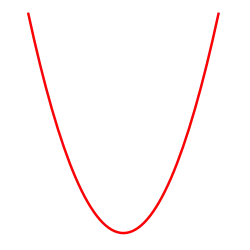
- the vanishing set is a parabola.
- this means
- the only solution is the point , the vanishing set is just a single point.
- this means
- the vanishing sets is the unit circle.
- again, this is empty.


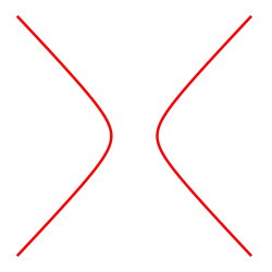
, the vanishing set consists in two lines crossing each other.


, the vanishing set is a hyperbola.


The polynomial does not appear directly in this list, because, in the variables and , we can write


In this form it is in the lists. The following theorem tells us that, up to scaling of the individual variables, the list is complete.
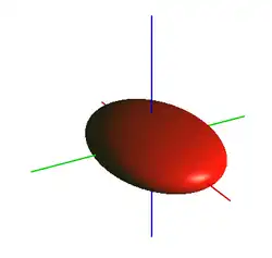
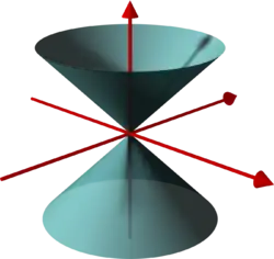
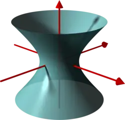
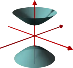
We make a list of real quadratic polynomials in the three variables and , together with their corresponding vanishing sets, where we restrict the coefficients to . Moreover, we consider only such polynomials where all variables occur and the vanishing set is not empty.


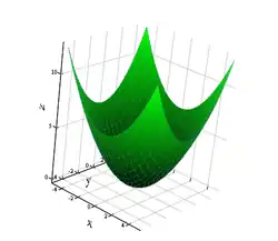
- the vanishing set is a paraboloid.
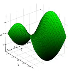
- the vanishing set is a saddle surface.
- the only solution is the point , the vanishing set is just one point.
- the vanishing set is a sphere, that is, the surface of a ball.
- the vanishing set is the solution set of the equation
- the vanishing set is a one-sheeted hyperboloid.
- the vanishing set is a two-sheeted hyperboloid.


. This is a (double)-cone.


Every real pure-quadratic polynomial

orthonormal basis (with respect to the standard inner product) the form


where

Using the matrix mentioned in the theorem we can write the polynomial in the form


By definition, the matrix is symmetric. Due to Theorem 42.12 , there exists an orthonormal basis of , such that the new Gram matrix


is a diagonal matrix, where

denotes the base change matrix from the new basis to the standard basis. We express this briefly as

in the sense of remark *****. Let be the dual basis of the new orthonormal basis. Thus, the describe the new coordinate functions, and we consider them as new variables. According to Lemma 14.14 , we have the relation


Therefore,

Calculating this yields , where the are the diagonal entries of . Because of Lemma 21.10 , the eigenvalues of and of are the same (and they have the same multiplicities).


We consider the pure-quadratic polynomial

In order to apply Theorem 43.10 , we have to find the eigenvalues of the matrix

The characteristic polynomial is

Therefore, the eigenvalues are

Therefore, in a suitable orthonormal basis, the polynomial has the form

We want to bring the pure-quadratic form

into a standard form in the sense of Theorem 43.10 . The corresponding symmetric matrix is

We have to determine the eigenvalues of this matrix. The characteristic polynomial of the matrix is

hence, the eigenvalues are

In the new variables for an orthonormal basis consisting of eigenvectors to these eigenvalues, we have


Every real quadratic polynomial

orthonormal basis (with respect to the standard inner product, and allowing translations), the form ( and )


or the form ( and )


We apply the transformation described in Theorem 43.10 to the pure-quadratic part . In the new variables (which are dual to the orthonormal basis), the polynomial has now the form


with a certain between and , and . The summands


can be brought, by completing the square and using new variables , to the form


Besides the pure-quadratic term, either a constant or a linear polynomial remains. In the second case, we denote this linear form by .

The representations occurring in this theorem are called the standard form of the quadratic form. In a standard form, we only have purely-quadratic terms and at most one variable in first degree. The theorem tells us that every quadratic form can be brought, using suitable orthonormal
(Cartesian)
coordinates, into such a standard form. Regarding the vanishing set, such a coordinate transformation means that we apply an affine-linear isometry.
A quadratic form in standard form

in the sense of Theorem 43.13 can be simplified further, if we allow distortions. In the new coordinates

or

for , the quadratic form has a representation of the form


the coefficients are or . This is called the normalized standard form of the quadratic form. By swapping of the variables, we may achieve that the first variables have the coefficient , and the later variables have coefficient . In doing these transformations, the vanishing sets are distorted. For example, an ellipse might become a circle, or a parabola might be compressed. Since the vanishing set does not change by multiplying the form with , we may also assume that the number variables with coefficient is at least the number of variables with coefficient .

We consider the quadratic polynomial

and we want to transform it according to Theorem 43.13 into a standard form. In Example 43.10 we have already studied the pure-quadratic part with the help of the symmetric matrix


the eigenvalues are
In order to transform itself to standard form, we need the eigenvectors, and we have to perform the change of variables explicitly. The eigenvectors are

therefore,

are an orthonormal basis consisting of eigenvectors. We have the relation

in the sense of remark *****. With den new variables we obtain according to Lemma 14.14 the relation


Hence, we obtain (for the pure-quadratic part, we do not have to compute anything)

By completing the square with

and

we get

and

Altogether this yields

| << | Linear algebra (Osnabrück 2024-2025)/Part II | >> PDF-version of this lecture Exercise sheet for this lecture (PDF) |
|---|