Linear algebra (Osnabrück 2024-2025)/Part II/Lecture 34
- Diagonalizability of isometries over the complex numbers
Let be a linear isometry on a finite-dimensional -vector space , endowed with an inner product. Let denote an invariant linear subspace. Then also the orthogonal complement is invariant. In particular, can be written as a direct sum


where the restrictions and
are also isometries.

We have

For such a and an arbitrary , we have


since due to the invariance of . Therefore, .


The following statement is called spectral theorem or, more specifically, spectral theorem for complex isometries. In this course, we will get to know further spectral theorems; see
Theorem 41.11
and
Theorem 42.9
.
Let be a finite-dimensional -vector space, endowed with an inner product, and let


be an isometry. Then has an orthonormal basis of eigenvectors of . In particular, is
diagonalizable.We do induction on the dimension of . The statement is clear in the one-dimensional case. Due to the Fundamental theorem of algebra and Theorem 23.2 , has an eigenvalue and an eigenvector, which we can normalize. Let be the corresponding eigenline. Since we have an isometry, the orthogonal complement is also, due to Lemma 34.1 , -invariant, and the restriction


is again an isometry. By the induction hypothesis, there exists on an orthonormal basis consisting of eigenvectors. Together with the first eigenvector, these form an orthonormal basis of eigenvectors of .
- Angles

For vectors and , different from , in a Euclidean vector space , the inequality of Cauchy-Schwarz implies that


holds. Using the trigonometric function cosine (as a bijective mapping ) and its inverse function, the angle between the two vectors can be defined, by setting
![{\displaystyle {}[0,\pi ]\rightarrow [-1,1]}](../../98e6b3005ba8d4d1af081eb25b71000609da4393.svg)

The angle is a real number between and . The equation above can be read as


This provides the possibility to define the inner product in this way. However, then we have to find an independent definition for the angle. This approach might look a bit more intuitive but has many disadvantages, computationally and in terms of the proofs.
For an affine space over a Euclidean vector space , and three given points (a triangle) with , the angle of the triangle at is the angle .


- Plane isometries
Let

be a proper linear isometry. Then is a rotation, and the describing matrix with respect to the standard basis has the form

with a uniquely determined rotation angle
.
Let and be the images of the standard vectors and . An isometry preserves the length of a vector; therefore,


Since an isometry preserves orthogonality, we have

In case , this implies (because of ) . Then , and, due to the properness assumption, the sign must be that of .


So let . Then


Since both vectors have the length , the modulus of the scalar factor is . In case , we had and the determinant was . Therefore, and . Hence, the describing matrix of with respect to the standard basis is


In particular, is a real number between and , and , that is, is a point on the real unit circle. The unit circle is parametrized by the trigonometric functions, that is, there exists a uniquely determined angle , , such that


The composition of two rotations
and
is . This property is intuitively clear, using intuitive properties of plane rotations. Using
the addition theorems
for the trigonometric functions, we can prove them. Moreover, the addition theorems follow from this property, see
Exercise 34.11
.
Therefore, the group of plane rotations is commutative.


Let
be an improper linear isometry. Then is an axis reflection, and its describing matrix, with respect to the standard basis, has the form

with a uniquely determined angle
.
We consider

which is by the multiplication theorem for the determinant a proper isometry. Because of Theorem 34.4 , there exists a uniquely determined angle such that


Therefore,

If such an axis reflection is given, then is an eigenvector for the eigenvalue , and the axis of reflection is ; see
Exercise 34.15
.
An axis reflection is described, with respect to the basis consisting of a vector of the reflecting axis and a corresponding orthogonal vector , by the matrix . This means that the description given in
Theorem 34.5
(with respect to the standard basis)
can be improved drastically.


- Isometries of space

The characteristic polynomial of is a normed polynomial of degree three. For , we have , and for , we have . Due to the intermediate value theorem, has a real zero. Such a zero is, according to Theorem 23.2 , an eigenvalue of . Because of Theorem 33.12 , this eigenvalue equals or .


A proper linear isometry of the space transforms the unit sphere into itself. One might imagine an isometry as a rotation of a ball lying in a suitable bowl.
eigenvector with eigenvalue , that is, there exists a line (through the origin)
that is a fixed line for .We consider the characteristic polynomial of , that is,

This is a normed real polynomial of degree three. For , we have


As the polynomial as , there must be a positive that is a zero of . Due to Theorem 33.12 , we must have .


Let
be a proper isometry. Then is a rotation around a fixed axis. This means that is described, with respect to a suitable orthonormal basis, by a matrix of the form

Due to Theorem 34.7 , there exists an eigenvector for the eigenvalue . Let denote the corresponding line. This line is fixed and, in particular, invariant under . Because of Lemma 34.1 , also the orthogonal complement is invariant under . That is, there exists a linear isometry


that coincides on with . Here, is proper. Therefore, by Theorem 34.4 , is a plane rotation. If we choose a vector of length one in , and an orthonormal basis of , then has with respect to this basis the given matrix form.

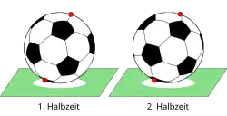
At the beginning of a football game, the football lies in the center spot. After a goal is scored, the ball is again put in the center spot. In this situation, the following holds: There exist at least two (antipodal) points on the ball (its surface)
that are at the new kick-off exactly at the position where they were at the first kick-off. The total movement of the ball is a rotation around an axis.The total movement is a linear isometry; therefore, the statement follows from Theorem 34.8 .
- The decomposition theorem for isometries
Let be a real finite-dimensional vector space, and let

denote an endomorphism. Then there exists a -invariant linear subspace of dimension
or .
We may assume , and that is described by the matrix with respect to the standard basis. If has an eigenvalue, then we are done. Otherwise, we consider the corresponding complex mapping, that is,


which is given by the same matrix . This matrix has a complex eigenvalue , and a complex eigenvector . In particular, we have


Writing

with , this means


Comparing the real part and the imaginary part we can deduce that . Therefore, the real linear subspace is invariant.


Let
be an isometry on the Euclidean vector space . Then is an orthogonal direct sum

of -invariant linear subspaces,
where the are one-dimensional, and the are two-dimensional. The restriction of to the is the identity, the restriction to is the negative identity, and the restriction to is a rotation without eigenvalue.


We do induction over the dimension of . The one-dimensional case is clear, due to Theorem 33.12 . Let . The determinant has, because of Lemma 33.13 either the value or . In case it is , the characteristic polynomial has two distinct zeroes, and these zeroes are, due to Theorem 33.12 , and . Then we have a reflection at an axis, and


If the determinant is , then we are in the situation of Theorem 34.4 , and we have a rotation. If the angle of rotation is , then we have the identity, and we can decompose . If the angle of rotation is , then we have a point reflection ; therefore, we have a decomposition . For all other angles, there is no eigenvector.


Let now be arbitrary, and suppose that the statement is proven for smaller dimensions. Because of Lemma 34.10 , there exists a -invariant linear subspace of dimension or , and, because of Lemma 34.1 , there exists an invariant orthogonal complement, that is,


The induction hypothesis, applied to , yields the result.

In this decomposition, is the eigenspace for the eigenvalue , and is the eigenspace for the eigenvalue ; the decompositions are not unique. The Isometry is proper if and only if is even.


| << | Linear algebra (Osnabrück 2024-2025)/Part II | >> PDF-version of this lecture Exercise sheet for this lecture (PDF) |
|---|