It is not the purpose of this page to repeat good information
available elsewhere.
However, it seems to the author that other descriptions of the cubic function are
more complicated than they need to be. This page attempts to
demystify elementary but essential information concerning the cubic function.
Objective
Present cubic function and cubic equation.
Introduce the concept of roots of equal absolute value.
Show how to predict and calculate equal roots, techniques that will be useful when applied to higher order functions.
The following python code implements the functionality of this section:
# python code.TwoRootsOfCubicDebug=0defTwoRootsOfCubic(abcd,x1):'''x2,x3 = TwoRootsOfCubic (abcd, x1)f(x2) = f(x3) = f(x1)If x1 is a root, then f(x2) = f(x3) = f(x1) = 0, and x2,x3 are roots.x1 may be complex.'''a,b,c,d=abcdB=a*x1+bC=B*x1+cdisc=B*B-4*a*CalmostZero=1e-15ifabs(disc)<almostZero:x2=x3=-B/(2*a)else:ifisinstance(disc,complex)or(disc>0):root=disc**.5else:root=((-disc)**.5)*1jx2=(-B-root)/(2*a)x3=(-B+root)/(2*a)ifnotTwoRootsOfCubicDebug:returnx2,x3sum1,sum2,sum3=[(a*x*x*x+b*x*x+c*x+d)forxin(x1,x2,x3)]print('TwoRootsOfCubic ():')print(' y = (',a,')xx + (',B,')x + (',C,')')print(' for x1 =',x1,', sum1 =',sum1)print(' for x2 =',x2,', sum2 =',sum2)print(' for x3 =',x3,', sum3 =',sum3)# sum1,sum2,sum3 should all be equal.# In practice there may be small rounding errors.# The following check allows for small errors, but flags# errors that are not "small".allEqualDebug=1allEqual((sum1,sum2,sum3))returnx2,x3
The 4 coefficients above are in fact the values
(same as above.)
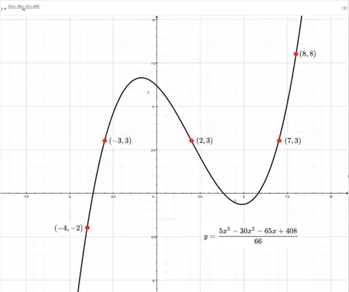
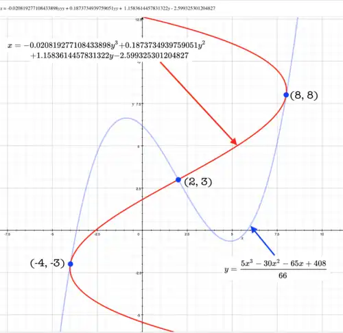
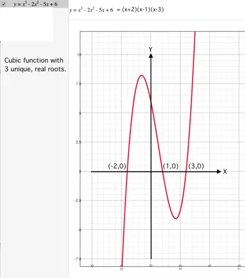
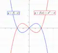
Graphs of 2 different cubic functions that satisfy the same 4 criteria.
If these 4 criteria (3 points and 1 slope) are used to define the cubic in which
is the independent variable, result is:
Both curves satisfy the points and have the same slope at point
(In fact )
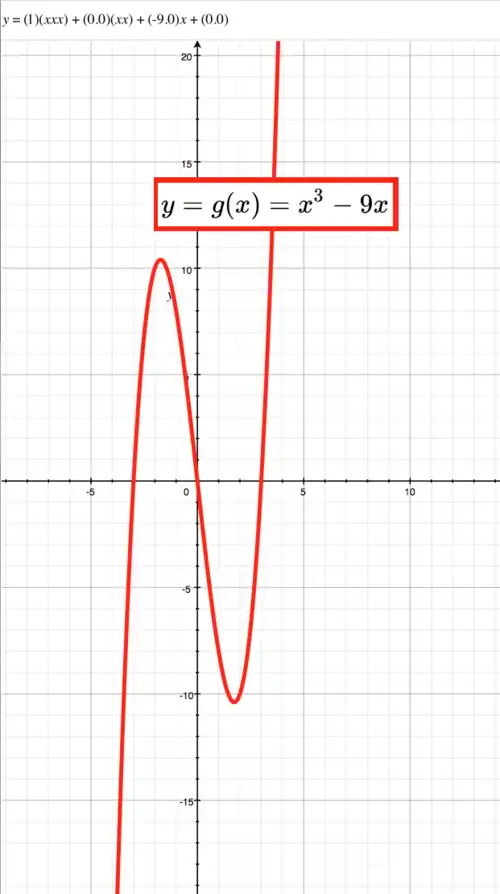
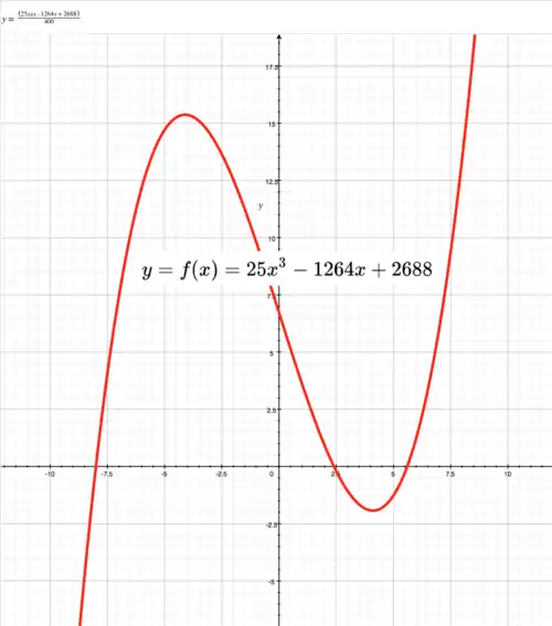
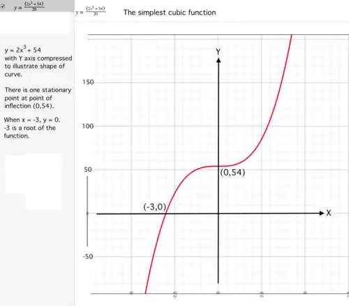
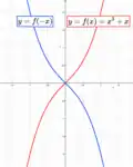
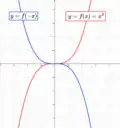
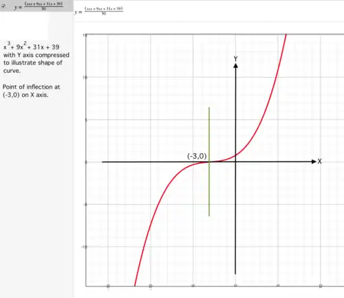
The simplest cubic function
Figure 1.
The simplest cubic function has coefficients
The simplest cubic function has coefficients , for example:
.
To solve the equation:
The function also contains two complex roots that may be found as solutions of the associated quadratic:
Curve is useful for finding the cube root of a real number.
Solve:
This is equivalent to finding a root of function
If you use Newton's method to solve it may be advantageous to put
in form where
Then Remember to preserve correct sign of result.
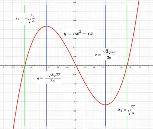
Roots of equal absolute value
The cubic function
Let one value of be and another be .
Substitute these values into the original function in and expand.
Reduce and and substitute for :
Combine and to eliminate and produce a function in :
From
If is a solution and function becomes:
and two roots of are .
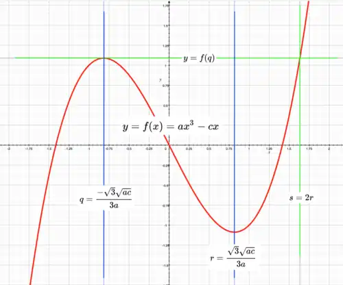
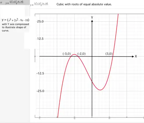
An example
Figure 2.
The roots of equal absolute value are
See Figure 2.
The function has roots of equal absolute value.
The roots of equal absolute value are .
This method works with complex roots of equal absolute value.
Consider function:
has roots of equal absolute value.
Roots of equal absolute value are:
Equal Roots
Combine and from above to eliminate and produce
a function in :
From above:
If , then is a solution ,
and become:
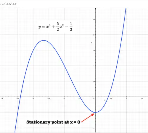
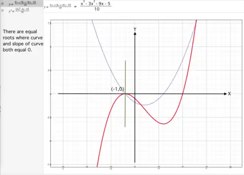
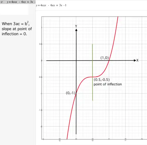
If because , there is a stationary point where .
Note:
is a factor of discriminant of cubic formula below. If because the discriminant is , function contains at least 2 roots equal to when both functions are .
are functions of the curve and the slope of the curve. In other words, equal roots occur where the curve and the slope of the curve are both zero.
and can be combined to produce:
and can be combined to produce:
If the original function contains 3 unique roots, then
are numerically different.
If the original function contains exactly 2 equal roots,
then are numerically identical, and the 2 roots
have the value in .
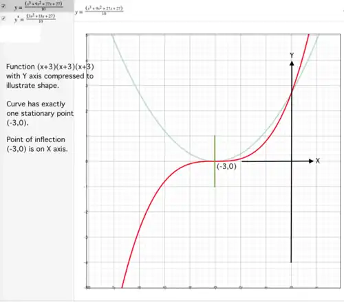
If the original function contains 3 equal roots, then
are both null, are numerically
identical and .
If contains 3 equal roots, and line t = w + C/w fails with divisor
Before using this formula, check for equal roots as in "3 equal roots" above.
Using cubic formula
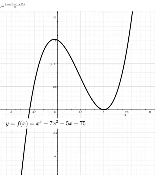
2 equal roots
Graph of cubic function with 2 equal roots at
Y axis compressed for clarity.
Calculate roots of
# python codea,b,c,d=1,-7,-5,75A=9*a*c-3*b*bB=27*a*a*d-9*a*b*c+2*b*b*bC=-A/3Δ=B*B-4*C*C*Cprint('Δ =',Δ)W=-B/2# The following 2 lines ensure that cube root of negative# real number is real number.ifW<0:w_=-((-W)**(1/3))else:w_=W**(1/3)r3=3**(0.5)values_of_w=(w_,w_*(-1+1j*r3)/2,w_*(-1-1j*r3)/2)forwinvalues_of_w:print()print('w =',w)t=w+C/wprint('t =',t)x=(-b+t)/(3*a)print('x =',x)
Δ = 0.0

w = -8
t = -16
x = -3

w = (4-6.928203230275509j)
t = 8
x = 5

w = (4+6.928203230275508j)
t = 8
x = 5
Notice that:
is zero.
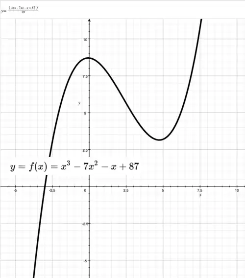
1 real root
Graph of cubic function with 1 real root at
Y axis compressed for clarity.
Δ = 1997568.0

w = -4.535898384862245
t = -16
x = -3

w = (2.2679491924311215-3.9282032302755088j)
t = (8.0+6.0j)
x = (5.0+2.0j)

w = (2.267949192431123+3.9282032302755083j)
t = (8.0-6.0j)
x = (5.0-2.0j)
Notice that:
is positive.
does not equal
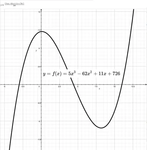
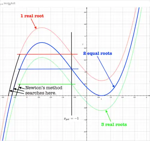
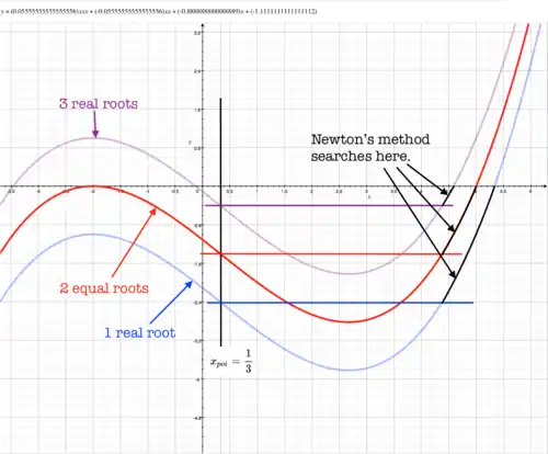
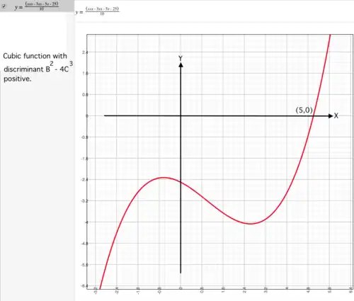
3 real roots
Graph of cubic function with 3 real roots,
Y axis compressed for clarity.
Δ = -197238264300.0

w = (51.5-32.042939940024226j)
t = 103
x = 11

w = (2.0+60.62177826491069j)
t = 4.0
x = 4.4

w = (-53.5-28.578838324886462j)
t = -107
x = -3
Notice that:
is negative
equals
cos (A/3)
The method above for calculating depends upon calculating the value of angle
However, may be calculated from
because
Generally, when is known, there are 3 possible values of the third angle because
This suggests that there is a cubic relationship between and
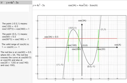
Expansion of cos (3A)
Figure 7a.
Graph of
The well known identity for is:
The derivation of this identity may help understanding and interpreting the curve of
Let
and
Therefore the point is on the curve and
A
3A
cos A
cos 3A
0
0
1
1
180
180*3
-l
-1
60
180
0.5
-1
Three simultaneous equations may be created from the above table:
Therefore
and
When is known,
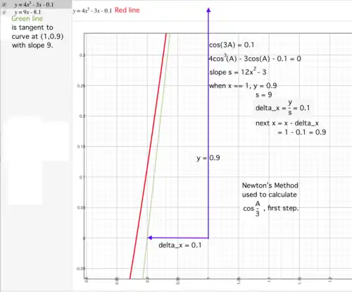
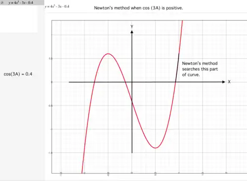
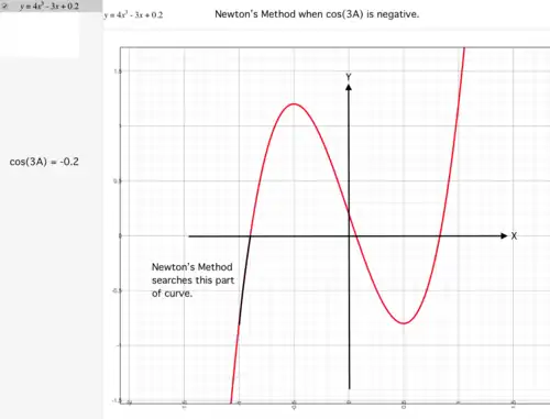
Newton's Method
Figure 7b.
Newton's Method used to calculate when
Newton's method is a simple and fast root finding method
that can be applied effectively to the calculation of when
is known because:
the function is continuous in the area under search.
the derivative of the function is continuous in the area under search.
the method avoids proximity to stationary points.
a suitable starting point is easily chosen.
See Figure 7b.
Perl code used to calculate when is:
$cos3A=0.1;$x=1;# starting point.$y=4*$x*$x*$x-3*$x-$cos3A;while(abs($y)>0.00000000000001){$s=12*$x*$x-3;# slope of curve at x.$delta_x=$y/$s;$x-=$delta_x;$y=4*$x*$x*$x-3*$x-$cos3A;print" x=$x y=$y ";}print" cos(A) = $x ";
The
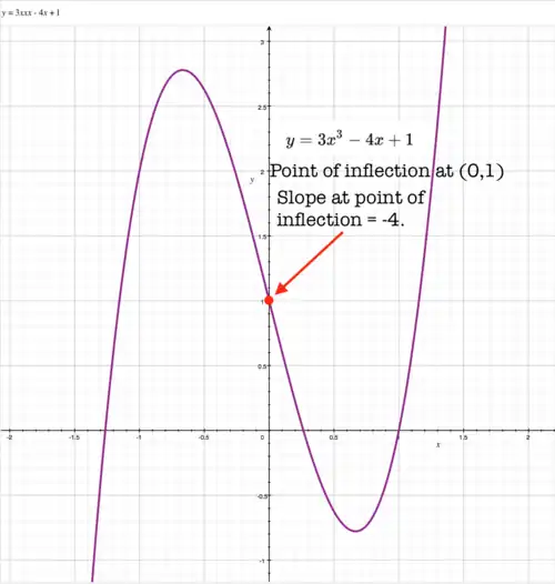
Point of Inflection
is the point at which the slope of the curve is minimum.
After taking the first and second derivatives value at point of inflection is:
The slope at point of inflection is:
Value at point of inflection is:
From basic principles
Figure 1. 4 points relative to point of inflection.
Relative to point of inflection :
Points have coordinates .
Points have coordinates .
When 2 points are equidistant in terms of they are also equidistant in terms of
may be calculated from basic principles.
Let us define the point of inflection as the point about which the curve is symmetric.
Let and let be non-zero.
Then where is point of inflection.
Let and
Then
Let be relative to
Then
Similarly
therefore:
Depressed cubic
Recall from "Depressed cubic" above:
Therefore:
Coefficients of the depressed cubic show immediately:
If slope at point of inflection is positive, zero or negative, and
If point of inflection is above, on or below X axis.
If 1 of is zero, the cubic equation may be solved as under
"Depressed cubic"
above.
Newton's Method
If both of the depressed function are non-zero,
Newton's method may be applied to the original cubic function, and the Point of Inflection
offers a convenient starting point.
When implemented as described below, Newton's Method always avoids that part of the curve where there might be equal roots.
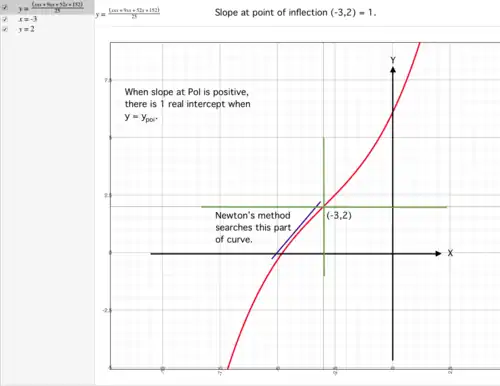
slope at PoI positive
Figure 8a.
Cubic function with positive slope at Point of Inflection
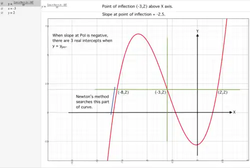
slope at PoI negative
PoI above X axis
Figure 8b.
Cubic function with negative slope at Point of Inflection
and PoI above axis.
When the other 2 intercepts may be calculated as roots
of the associated quadratic with coefficients:
Graphs of 3 different cubic functions all solved with the same technique.
The figure shows all possible considerations if point of inflection is above
axis.
The same technique using Newton's Method works well with all conditions.
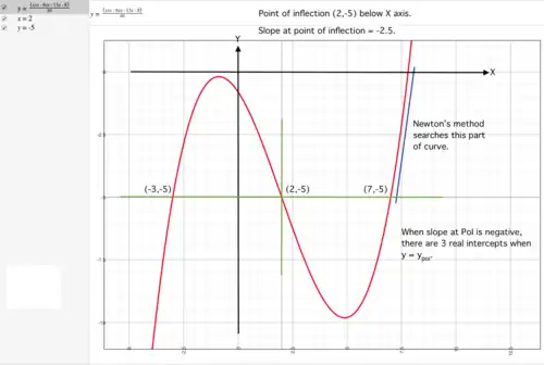
PoI below X axis
Figure 8c.
Cubic function with negative slope at Point of Inflection
and PoI below axis.
When the other 2 intercepts may be calculated as roots
of the associated quadratic with coefficients:
Graphs of 3 different cubic functions all solved with the same technique.
The figure shows all possible considerations if point of inflection is below
axis.
The same technique using Newton's Method works well with all conditions.
Using Newton's method
The method used to solve the cubic equation (as presented here) depends on the value of the discriminant
(B² - 4C³). If this value is non-negative, the value of 1 root is easily calculated and the other 2 roots
are solutions of the associated quadratic described under
"linear and quadratic"
above.
If this value is negative, the use of this value leads to some interesting theory of complex numbers and the solution
depends on the calculation of
The method above uses Newton's method to calculate
from
Newton's method is very fast and more than adequate to do the job. However, the purist might say that the solution of
a cubic equation must not depend on the solution of a cubic equation. The solution offered under
"Cosine(A/3)"
above satisfies the purist.
Also, if you're going to use Newton's method to calculate why not use Newton's
method to calculate one real root of the original cubic?
One of the objectives above is to show that the cubic equation can be solved with high school math.
Newton's method can be implemented with a good knowledge of high school calculus and the starting point may depend on
the solution of a quadratic equation, also understood with a good knowledge of high school algebra.
The example presented below shows how to solve the cubic equation with high school math.
For function TwoRootsOfCubic() see General_case above.
Calculate roots of cubic function:
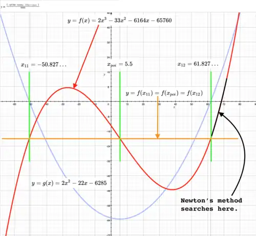
# python codea,b,c,d=abcd=2,-33,-6164,-65760# Coefficients of depressed cubic:A=9*a*c-3*b*bB=27*a*a*d-9*a*b*c+2*b*b*b# The point of inflection:ypoi=B/(27*a*a)xpoi=-b/(3*a)spoi=A/(9*a)print('xpoi =',xpoi)print('ypoi =',ypoi)print('spoi =',spoi)
xpoi = 5.5
ypoi = -100327.5
spoi = -6345.5
is negative. will not be used as starting point.
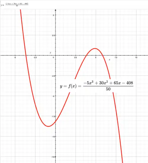
Figure 1: Diagram illustrating relationship between and
Roots of are 2 possible starting points.
Because is below axis, is chosen.
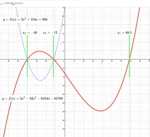
The associated quadratic when
Find 2 possible starting points to left and right of
The starting point start is close to which was found quickly.
If only one root is required (as in calculation of roots of quartic function), may be used,
in which case calculations below are not necessary. The big advantage of using
is that is guaranteed to be a real number.
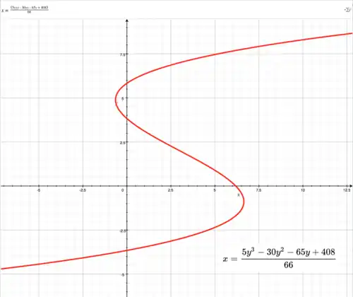
Figure 2: Diagram illustrating relationship between and Roots of are 2 roots of
Much interesting theory concerning complex numbers and Vieta's substitution has been presented above.
The formula for a root of the cubic equation, is already appearing to be too complicated.
Using the formula usually involves calculation of square root and cube root, possibly a complex cube root.
How are these values calculated? Possibly by using Newton's method.
Every cubic function is guaranteed to contain at least one real root. The function below,
oneRootOfCubic (), is an attempt at almost extreme simplicity.
Considerations such as equal roots or complex cube root are ignored.
After a few simple decisions, Newton's method is used to derive one real root of the given cubic.
# Python codenewtonDebug=0defnewton(abcd,startx):'''x = newton (abcd, startx)Values a,b,c,d,startx may be Decimal or non-Decimal, but not a mixture of both.x is float or None.Newton's method for finding 1 root of cubic function.2 global variables are needed: newtonDebug almostZero (same as relative tolerance)'''ifnewtonDebug:print('newton() 1: a,b,c,d =',abcd)a,b,c,d=abcdx=startx;xx=x*xy=a*xx*x+b*xx+c*x+difnewtonDebug:print('newton() 2: x,y =',x,y)# The differential function# slope = 3*a*x*x + 2*b*x + c_a=3*a_b=2*b_c=ccount=0;L1=[]while1:count+=1ifcount>=51:print('newton() 3: count expired.')returnNoneslope=_a*xx+_b*x+_cdelta_x=y/slopex-=delta_xxx=x*xt3,t2,t1=a*xx*x,b*xx,c*xy=t3+t2+t1+d# Yes. This calculation of y is slightly faster than:# y = a*x*x*x + b*x*x + c*x + difnewtonDebug:print('newton() 4: x,y =',x,y)ifabs(y)<=almostZero:breakmax=sorted([abs(v)forvin(t3,t2,t1,d)])[-1]ifabs(y)/max<=almostZero:breakifxinL1[-1::-1]:ifnewtonDebug:print('newton() 5: Endless loop detected.')returnNoneL1+=[x]ifnewtonDebug:print('newton() 6: count =',count)returnx
# Python codeimportdecimalD=decimal.DecimaloneRootOfCubicDebug=0defoneRootOfCubic(abcd):'''x1 = oneRootOfCubic (abcd)Each member of a,b,c,d must be int or float or Decimal.If any member is Decimal, this function ensures that all are Decimal.x1 may be None.'''useDecimal=Falseforvinabcd:ifisinstance(v,D):useDecimal=True;continueiftype(v)notin(int,float):print('oneRootOfCubic() 1: Each member of input (abcd) must be int, float or Decimal.')returnNoneifuseDecimal:a,b,c,d=[D(str(v))forvinabcd]else:a,b,c,d=abcdifa==0:print('oneRootOfCubic() 2: a must be non-zero.')returnNoneifd==0:return0ifa!=1:divider=aa,b,c,d=[v/dividerforvin(a,b,c,d)]# a is now +1.ifb==c==0:# This is effectively the calculation of cube root.ifoneRootOfCubicDebug:print('oneRootOfCubic() 3: Cube root of',-d)root3=simpleCubeRoot(-d)ifuseDecimal:returnD(str(root3))returnfloat(root3)xpoi=-b/3# Point of inflection.# Coefficient B of depressed cubic. B = 27*a*a*d - 9*a*b*c + 2*b*b*bB=27*d-9*b*c+2*b*b*bifB==0:# Point of inflection is on X axis.ifoneRootOfCubicDebug:print('oneRootOfCubic() 4: Found B=0.')returnxpoiA=3*c-b*b# Coefficient A of depressed cubic. A = 9*a*c - 3*b*bifA==0:# Slope at Point of inflection is 0.ifoneRootOfCubicDebug:print('oneRootOfCubic() 5: Found A=0.')t=simpleCubeRoot(-B)ifnotuseDecimal:t=float(t)x=(-b+t)/3returnxifA>0:# Slope at Point of inflection is positive.returnnewton((a,b,c,d),xpoi)# Slope at Point of inflection is negative.x1,x2=TwoRootsOfCubic([float(v)forvin(a,b,c,d)],float(xpoi))ifoneRootOfCubicDebug:print('oneRootOfCubic() 6: x1,x2 =',x1,x2)ifuseDecimal:x1,x2=[D(str(v))forvin(x1,x2)]ifB>0:# Point of inflection is above X axis.returnnewton((a,b,c,d),x1)# Point of inflection is below X axis.returnnewton((a,b,c,d),x2)
For function TwoRootsOfCubic () see General case above.
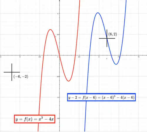
Graphs of 2 cubic functions with same shape.
Red curve relative to point is same as blue curve relative to
The familiar equation of the cubic function: This is the equation of
relative to origin However, need not be constrained as always
relative to origin. It is always possible, and sometimes desirable, to express relative to any other point in the two dimensional plane. The process of producing a new function
that is relative to is called "Translation of axes."
On this page the point of reference of any cubic function is the point of inflection.
Point of inflection of (red curve) is Relative to point
red curve is located at Relative to blue curve is located at
and equation of blue curve is or
Equation of relative to is:
where:
Move cubic function to (u,v)
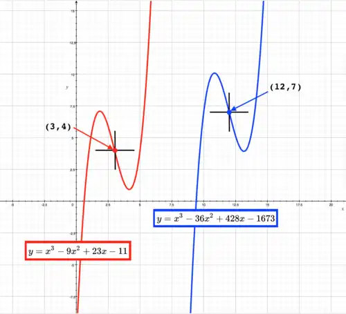
Graphs of 2 cubic functions with same shape.
Red curve moved to has equation
Blue curve moved to has equation
When a cubic function is moved to point the point of inflection is moved from present position
to and the amount of movement is:
Equation of function after being moved is:
or where:
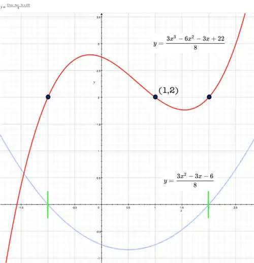
Describing a cubic function
Graph of complicated cubic function simplified.
Given a random cubic function, particularly those with large coefficients, it's usually difficult to visualize the function. One way to simplify our perception of a random cubic function is to
consider the function at origin This can be done by:
moving function to or
calculating equation of function relative to point of inflection


![{\displaystyle x={\sqrt[{3}]{-27}}=-3}](./88e7ae12347d5209e02e0e1372ba1b7d77c10cb2.svg)


![{\displaystyle x={\sqrt[{3}]{N}}.}](./84711cc10042a70032e740db3611a059f2178ef0.svg)


![{\displaystyle {\sqrt[{3}]{N}}={\sqrt[{3}]{n}}(10^{p}).}](./786877600e76960e33522dd217bf89309ba26510.svg)


![{\displaystyle t={\sqrt[{3}]{216}}=6}](./14e91a3b6d85d6943d13663924846efbd9d2a342.svg)


![{\displaystyle w={\sqrt[{3}]{W}}}](./c32e82fa13f8e647f58092d72706da6bfac2d815.svg)


![{\displaystyle w={\sqrt[{3}]{216}}=6}](./ad0534eabc066849c7fa19d480e9c12c40e33b76.svg)


![{\displaystyle w={\sqrt[{3}]{W}}=9.464101615137753}](./a55efff9547c6344b86160722c450f33de7b31ee.svg)


![{\displaystyle w={\sqrt[{3}]{W}}=2.5358983848622447}](./f7b20406a257f7806311be0327c97b7f61b72646.svg)


![{\displaystyle w_{mod}={\sqrt[{3}]{W_{mod}}}={\sqrt {C}}}](./ad57a7d0e7739c4ae7497c3fc58a288fffdf2b96.svg)


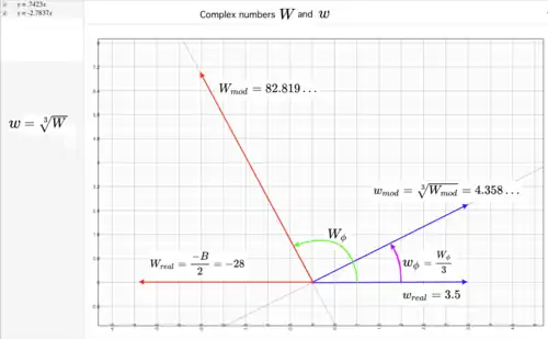


![{\displaystyle w_{mod}={\sqrt[{3}]{W_{mod}}}}](./d06430a1303a913ce7b37d5b6b3d7633d32edbc4.svg)


![{\displaystyle x={\frac {-b+{\sqrt[{3}]{\frac {-(27a^{2}d-9abc+2b^{3})+{\sqrt {(27a^{2}d-9abc+2b^{3})^{2}-4(b^{2}-3ac)^{3}}}}{2}}}+{\frac {(b^{2}-3ac)}{\sqrt[{3}]{\frac {-(27a^{2}d-9abc+2b^{3})+{\sqrt {(27a^{2}d-9abc+2b^{3})^{2}-4(b^{2}-3ac)^{3}}}}{2}}}}}{3a}}}](./264b2fee261735044a3f1be226a0cfbac994ac40.svg)

![{\displaystyle {\sqrt[{3}]{W}}}](./5a64d1bc536103c3db92a62c008b0361858b394e.svg)