What maximizes entropy?

Question

Liouville theorem states that the phase space distribution function of a system remains unchanged with the system evolution, $$ \frac{\text{d}\rho}{\text{d}t}=\frac{\partial \rho}{\partial t}+\sum_{i=1}^N\left(\frac{\partial \rho}{\partial q_i}\dot{q}_i+\frac{\partial \rho}{\partial p_i}\dot{p}_i\right)=0. $$ A consequence of this is that any function of the distribution function also remains unchanged. Specifically, this is true for entropy, defined as $$ S_G=-\int \rho(\mathbf{q},\mathbf{p},t)\log\left[\rho(\mathbf{q},\mathbf{p},t)\right] \prod_{i=1}^N\text{d}q_i \text{d}p_i. $$ The entropy here is Gibbs II entropy (similar to Shannon entropy), but not Boltzmann-Einstein-Planck entropy $S_{BEP}=k_B\log W$, which corresponds to the equal occupation of microstates and equals to Gibbs II only when thermodynamic equilibrium distribution function is assumed.

Thus, if we start with a system out of equilibrium, it would never evolve towards the maximum entropy state. The usual reasoning in Statistical Mechanics texts is that a system evolves towards equilibrium due to residual interactions that we otherwise neglect in equilibrium - e.g., collisions between molecules, which we ignore when discussing an ideal gas. But Liouville theorem then states that no internal interactions can produce such a relaxation.

How is this resolved (in theory and in practice)? Should we necessarily assume interaction with an environment (and is it enough)?

Background: the question motivated by this discussion: Are there known conditions that ensure infinite slowness is reversible?

Answer 1

This is an old question but, as with everything about entropy, the issue keeps coming back. Jaynes addressed it in 1965 and gave a nice explanation of the fact that the Liouville equation and Gibbs's definition of entropy are not at odds with each other. I will take a somewhat broader view of the perceived problem ans especially of the limitations of the Liouville equation.

It is well known that the Liouville equation is isentropic, i.e., it preserves whatever entropy the ensemble was given at $t=0$. This is not the paradox that it sounds. The reason is that the Liouville equation does not describe the relaxation of the ensemble from arbitrary initial state to final equilibrium. In fact, it cannot describe relaxation because it is based on deterministic classical mechanics. Even though the Louisville equation takes as input a probabilistic initial condition, specified by the distribution of microstates at $t=0$, it evolves these states deterministically. Every microstate at $t_0$ evolves to a new and distinct microstate at $t=t_0 + \Delta t$, the number of microstates is preserved, hence entropy is constant. This is a shortcoming of the Liouville equation, not of the Gibbs entropy, as often is argued by some.

We should not conclude from this...

Thus, if we start with a system out of equilibrium, it would never evolve towards the maximum entropy state.

The correct conclusion is

We cannot use the Liouville equation to identify the equilibrium state of the ensemble. We can only use to examine how the equilibrium state might evolve in time. In other words, the Liouville equation is a necessary but not sufficient condition on the equilibrium probability distribution.

It is instructive to examine how Gibbs used the Liouville equation. First he showed that if the probability distribution $\rho(\Gamma)$ of microstate $\Gamma$ is an explicity function of the Hamiltonian rather than of the microstate, i.e., $$ \rho(\Gamma) = \rho(\mathcal H) $$ with $\mathcal H=\mathcal H(\Gamma)$, then the Liouville equation is still satisfied. So, rather than searching for a function $\rho(\Gamma)$ with $\Gamma = (q_1,\cdots,q_N; p_1\cdots,p_N)$ where $N$ is an impossibly large number of degrees of freedom, we might as well search for a function $\rho(\mathcal H)$ of a single variable, $\mathcal H$.

Gibbs went on to guess the canonical partition function:

The distribution represented by \begin{equation}\tag{90} \eta=\log P = \frac{\psi-\epsilon}{\Theta}, \end{equation} or \begin{equation}\tag{91} P = e^{\dfrac{\psi-\epsilon}{\Theta}}, \end{equation} where $\Theta$ and $\psi$ are constants, and $\Theta$ positive, seems to represent the most simple case conceivable [the emphasis in mine], since it has the property that when the system consists of parts with separate energies, the laws of the distribution in phase of the separate parts are of the same nature, a property which enormously simplifies the discussion, and is the foundation of extremely important relations to thermodynamics. The case is not rendered less simple by the divisor $\Theta$, (a quantity of the same dimensions as $\epsilon$,) but the reverse, since it makes the distribution independent of the units employed. The negative sign of $\epsilon$ is required by (89), which determines also the value of $\psi$ for any given $\Theta$, viz., \begin{equation}\tag{92} e^{-\frac{\psi}{\Theta}} = \idotsint\limits_\text{phases}^\text{all} e^{-\frac{\epsilon}{\Theta}}dp_1\cdots dq_n .\end{equation} Gibbs, Elementary Principles of Statistical Mechanics, p33

In other words Gibbs did not derive the canonical probability from the Liouville, equation, he guessed it. He used the necessary condition provided by the Liouville equation to narrow the search, but at the end the distribution had to be guessed. Of course, after guessing its form Gibbs goes on in the rest of his book to show that this distribution makes thermodynamic sense.

Answer 2

Here is an interesting but longish quote from Pippard: ELEMENTS OF CLASSICAL THERMODYNAMICS, pp96-98, that is, I believe, in agreement with the statistical interpretation of Jaynes (especially his end comments regarding the anthropomorphic nature of entropy):

Now for any given set of constraints a thermodynamic system has only one true equilibrium state, and we may therefore formulate the entropy law in a slightly different way:

It is not possible to vary the constraints of an isolated system in such a way as to decrease the entropy.

This formulation focuses attention on the constraints to which a system is subjected, and it is instructive to follow up this line of argument in connexion with the fluctuations which are an essential feature of the equilibrium state. To make the meaning clear we shall consider a specific example, the second of the three mentioned above, in which a gas is released from a smaller into a larger volume. When the gas is in equilibrium in the larger volume its density is very nearly uniform, but is subject to continual minute fluctuations. Very occasionally larger fluctuations will occur, and there is a continuous spectrum of possible fluctuations ranging, with decreasing probability, from the very small to the very large; so that it is a theoretical possibility (though it is overwhelmingly improbable of observation even on a cosmic time scale) that the gas may spontaneously collapse into the smaller volume from which it originally escaped at the piercing of the wall. It will subsequently expand again to fill the full volume at just the same rate as at the first escape. We may now inquire what happens to the entropy of the gas during this large-scale fluctuation, and to this question the only satisfactory answer is the perhaps surprising one - nothing. For the continuous spectrum of fluctuations of all magnitudes is, as stressed before, part of the nature of thermodynamic equilibrium; the huge fluctuation just envisaged does not represent a departure from equilibrium - it is simply an extremely rare configuration of the gas molecules, but still just one of the enormous number of different configurations through which the gas passes in its state of equilibrium subject to given constraints. If we ascribe a definite value to the entropy of the gas in equilibrium we must ascribe it not to any particular, most probable, set of configurations, but to the totality of configurations of which it is capable. Thus we see that the entropy (and of course other thermodynamic functions) must be regarded as a property of the system and of its constraints, and that once these are fixed the entropy also is fixed. Only in this sense can any meaning be attached to the statement that the entropy of an isolated mass of gas, confined to a given volume, is a function of its internal energy and volume, S=S(U, V). It follows from this that when the gas is confined to the smaller volume it has one value of the entropy, when the wall is pierced it has another value, and that it is the act of piercing the wall and not the subsequent expansion that increases the entropy. In the same way when two bodies at different temperatures are placed in thermal contact by removal of an adiabatic wall, it is the act of removing the wall and not the subsequent flow of heat which increases the entropy. It will be seen then that our second statement of the entropy law has much to recommend it in that it concentrates upon the essential feature of a thermodynamic change, the variation of the constraints to which a system is subjected.

To take this argument to its ultimate logical conclusion leads to a rather curious situation. Since no walls are absolutely impervious to matter or to heat we may consider that no constraints are perfect; no two bodies in the universe are absolutely incapable of interaction with one another. Therefore the entropy of the universe is fixed once and for all, and the present state of the universe either is, or for thermodynamic purposes simulates, an enormous fluctuation from the mean state of more or less uniform density and temperature. But, apart altogether from the entirely unjustifiable assumption that the universe can be treated as a closed thermodynamic system, this point of view is not very useful, since it makes it difficult, if not impossible, to apply the entropy law in any situation. It is better by far to make a reasonable compromise, of the same nature as those which we made in Chapter 2. Although truly adiabatic walls do not exist, we imagine for the sake of argument that they do, so that small portions of the universe may be considered in isolation. A similar compromise was involved in our discussion of metastability, in which we concluded that no harm would arise from assuming that reactions which proceed immeasurably slowly are not proceeding at all. We are then enabled to define the entropy of physically interesting systems, and apply the entropy law to them without difficulty.

Answer 3

This is quite difficult to explain. I would say that this animation is the short explanation. Now I'm getting into the long explanation. This is an extract from a text I have written recently. I use the letter $\mu$ instead of $\rho$ but they mean the same. For me, distribution and macrostate are synonyms. Everything is explained with classical mechanics but I guess the ideas would be very similar in quantum mechanics.

The mechanical transformation of the system is a change in time of the external parameter $V$, a function $V(t)$ defined on some internal $[t_0,t_1]$. The Hamiltonian changes accordingly:

$$H(t)=H(V(t))$$

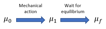
A system is initially in an equilibrium state $\mu_0$. After the transformation, the system is now in state $\mu_1$. Assume the change is irreversible. $\mu_1$ is not an equilibrium state. According to Liouville's theorem, Gibbs entropy is preserved:

$$S(\mu_0)=S(\mu_1)$$

Why then, do we say entropy increases? Strictly speaking, entropy has not increased yet.

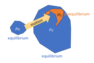
For simplicity, we are going to describe the phenomenon as if macrostates were subsets of the phase space (rather than distributions) like microcanonical ensembles. $\mu_1$ might be a “subset” of a larger equilibrium macrostate. After the transform is finished, the system keeps on following motion on its own, following its natural trajectories at constant energy. Since we assume the system is ergodic, from a given microstate the system can visit any other microstate of the same energy level. Call $\mu_f$ the union of all trajectories intersecting $\mu_1$. If we let the system follow motion on its own, it starts visiting $\mu_f$. When $\mu_1$ is not an equilibrium state:

$$S(\mu_f)>S(\mu_1)$$

The process has somehow two steps:

If you imagine the states as subsets of the phase space, it looks like it:

We said that when the equilibrium is restored, $\mu_1$ becomes $\mu_f$. But what exactly means “the equilibrium is restored”? Is there a true physical reality such as “equilibrium is restored”? An equilibrium state is when our knowledge does not vary with time. But unless we decide to be amnesiac, it clearly does.

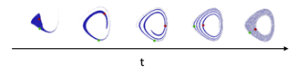
Write $f_t$ the Hamiltonian flow (the motion) at $V(t_1)$. At time $t_1$ the distribution is $\mu_1$ and later, at time $t+t_1$ it is $f_t(\mu_1)$. The true distribution constantly changes and because of Liouville’s theorem, it has constant entropy $S(μ_1)$. If we had to describe how $f_t (\mu_1)$ evolves, it sorts of begins to “fill” $\mu_f$ so that at some point, it seems to cover $\mu_f$. No practical experiment will soon be able to tell $f_t(\mu_1)$ from $\mu_f$. The information never disappears but becomes lost in a mess of extreme complexity, so that no realistic experiment can tell the real state from the equilibrium one. The property we just described is unproven. It is a hypothesis stronger than the ergodic hypothesis. In the language of ergodic theory, it is close to a property called mixing. Mixing implies that $f_t(\mu_1)$ becomes a messy shape undistinguishable from the larger $\mu_f$. Something like this:

Theoretically, it is not even true that mixing prevents going back to $\mu_1$ and really justifies what we said. Mixing is only an asymptotic property. Visually, it looks like $f_t(\mu_1)$ fills $\mu_f$ but before $t=+\infty$, it does not provably prevent exploiting the information that we were in $\mu_1$. If a device was capable to revert all atoms velocities instantaneously, we could revert motion back to $\mu_1$. I am not aware of any limitation of mechanics preventing such a device to exist in some way, even if totally unrealistic.

Answer 4

One way to explain this (or at least to kick the can down the road) is by invoking the assumption of ergodicity. If we claim that over its time evolution the system explores all the possible states, and visits every point of the phase space equally frequently, then its time averaged distribution function tens to a constant on a hypersurface of accessible states: $$ \overline{\rho(\mathbf{q},\mathbf{p},t)}^T=\frac{1}{T}\int_{t_0}^{t_0+T}\rho(\mathbf{q},\mathbf{p},t)\text{d}t\longrightarrow W^{-1}\text{ as } T\rightarrow +\infty $$ We then get the BEP entropy as that calculated using this time averaged probability density.

In practice this means that the time of observation should be sufficiently long for the system to visit most of the typical states of the system, so that the observations resemble the ensemble average obtained with many systems starting from different initial conditions.

A couple of further comments:

• A single classical system is always in a single configuration, i.e., it is inherently non probabilistic. Thus, without time averaging it probably doesn't even make sense to talk about its entropy. It would seem less striking, if we talked about a quantum system, which can be in several states simultaneously - but it is simply because the ensemble averaging is already implied in quantum mechanics, and the problem is pushed from interpreting statistical physics to interpreting the QM.
• The situations where the observation time is not sufficiently long for the system to visit all the likely configurations are also well-known in the domain of critical phenomena, such as, e.g., the polarization of a ferromagnet. - phase transitions