I am not good at Physics so please bear with me. I am trying to understand harmonics and in order to do that I thought its best to ensure my understanding of the equations of motion is correct. To do this I tried to model a mass vibrating on a frictionless surface with restoring force from a spring when acted on by a force F. The parameters are as follows:
M = 5 kg (Mass)
F = 10 kN (Initial force)
k = -1kN/m (Spring constant)
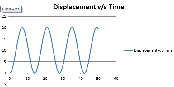
I expected the plot of displacement against time to be uniform i.e without dissipation (or no damping). However, the result shows that the displacement are increasing. Have I made a mistake, if not, could someone explain the phenomena.
The plot is shown below
Algorithm is as follows:
F = 10kN
m = 5kg
k = -1kN/m
initial acceleration, a0 = 10/5 = 2 m/s

Assuming displacement is positive to the right
    At t = 0,
    u = 0
    v = 0
    s = 0
    dt = 1
    a0 = 2
    ar = 0
    anet= a0-ar
    While (t<100),
       ds = u*dt + 0.5anet*dt^2;
       s = s + ds;
       v = u + anet*dt;
       t = t + dt
       acceleration by restoring force, ar= (k*s/m);
       updating net acceleration, anet = anet + ar; //K is already negative
    Next;
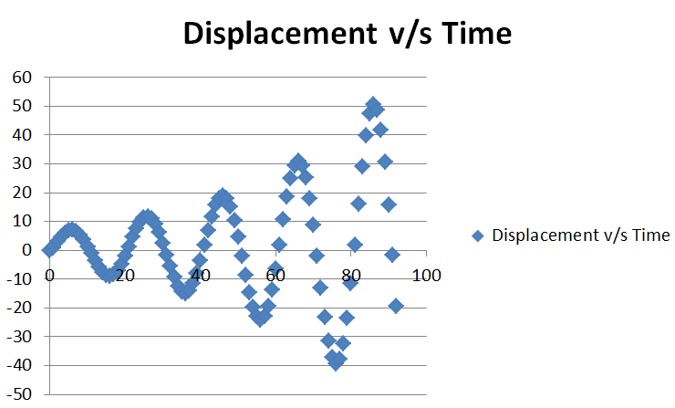
Update: I plotted the same graph at different time steps.
TimeStep=0.1s
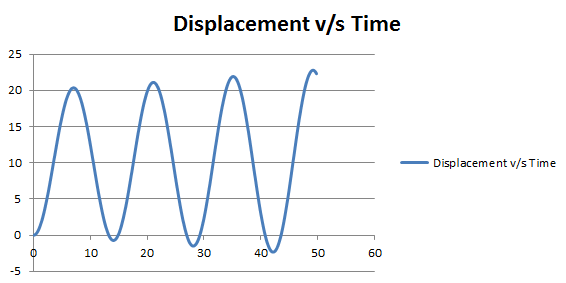
TimeStep=0.005s